Cross-validating EcoCommons SDM outputs against reference implementations (on development)

Author details: Xiang Zhao

Contact details: support@ecocommons.org.au

Copyright statement: This script is the product of the EcoCommons platform. Please refer to the EcoCommons website for more details: https://www.ecocommons.org.au/

Updated date: 8 September 2026

Script information

This page documents the scientific-agreement unit tests that guard every species distribution model (SDM) algorithm on the EcoCommons platform. Each test runs a real EcoCommons projection and compares it against an independent reference implementation — the algorithm’s own R package, Valavi et al. (2021)’s published benchmark on the NCEAS nsw14 data, the reference implementations in Hijmans & Elith’s Species distribution modeling with R (the dismo vignette), or our verbatim reproduction of Guisan, Thuiller & Zimmermann’s Habitat Suitability and Distribution Models (2017) on the Vulpes vulpes data (for SRE, FDA, ANN, GBM, GLM, GAM, MARS and CTA).

Every SDM agreement test in the EcoCommons R package (tests/testthat/test-sdm_projection_agreement.R) runs a real EcoCommons projection and compares it to a reference benchmark — the algorithm’s own R package, Valavi et al. (2021)’s published benchmark on the NCEAS nsw14 data, or our HSDM (Guisan et al. 2017) Vulpes vulpes reproduction.

Algorithm coverage

EcoCommons ships 19 species-distribution / geographic algorithms. 17 are guarded by a scientific-agreement unit test (SRE, FDA, ANN, GBM, GLM, GAM, MARS and CTA covered against the HSDM Vulpes vulpes reproduction — ANN as a 50× ensemble, a deliberate change from the book’s single fit); 2 are not yet covered.

Family	Algorithm	EcoCommons engine	Sci Unit Test?
biomod2 SDMs	GLM	stats::glm	✅ tested
	GAM	mgcv::gam	✅ tested
	RF	randomForest	✅ tested
	MARS	earth	✅ tested
	GBM	gbm	✅ tested
	CTA	rpart	✅ tested
	FDA	mda	✅ tested
	ANN	nnet	✅ tested
	SRE	biomod2 (envelope)	✅ tested
dismo SDMs	MaxEnt	maxent.jar	✅ tested
	BRT	dismo::gbm.step	✅ tested
	Bioclim	dismo::bioclim	✅ tested
Geographic (spatial-only)	GeoDist	dismo::geoDist	✅ tested
	Convex Hull	dismo::convHull	✅ tested
	Circles	dismo::circles	✅ tested
	GeoIDW	dismo::geoIDW	✅ tested
	Voronoi Hull	dismo::voronoiHull	✅ tested
Niche / match	Range bagging	ecospat-style range bagging	❌ not yet
	Climatch	climate-matching	❌ not yet

Sci-unit-tested (17): GLM, GAM, RF, MARS, MaxEnt, BRT, Bioclim, GeoDist, Convex Hull, Circles, GeoIDW, Voronoi Hull, SRE, FDA, ANN, GBM, and CTA. Not yet covered (2): Range bagging, Climatch. (The speciestrait_* / traitdiff_* trait-difference functions are out of scope here — they are not species-distribution models.)

Overview — all tests, grouped by model family

Every test runs a real EcoCommons projection and scores it against a reference implementation on Pearson (or Spearman rank, for tie-heavy CTA) correlation of predicted suitability. Rows are grouped by algorithm family (Profile · Machine Learning · Statistical · Geographic); the two algorithms not yet covered (Climatch-lite, Range Bagging) are shown in their family for completeness.

#	Algorithm	Species	EcoCommons engine	Reference benchmark	Metric	Threshold	Result
Profile Models
1	BIOCLIM	Bradypus variegatus	dismo::bioclim	dismo bioclim	Pearson	0.90	0.980 ✓
—	Climatch-lite	—	climate-matching	—	—	—	❌ not yet
—	Range Bagging	—	ecospat-style range bagging	—	—	—	❌ not yet
2	Surface Range Envelope (SRE)	Vulpes vulpes	biomod2 bm_SRE	HSDM (Guisan et al. 2017) reproduction	Pearson	0.99	1.000 ✓
Machine Learning Models
3	Artificial Neural Network (ANN)	Vulpes vulpes	biomod2 nnet (50× ensemble)	HSDM reproduction (50× ensemble)	Pearson	0.95	0.996 ✓
4	Boosted Regression Tree (BRT)	Anguilla australis	dismo::gbm.step (unit weights)	dismo gbm.step (unit weights)	Pearson	0.95	0.985 ✓
5		nsw14	dismo::gbm.step (test mocks down-weighting)	gbm.step (down-weighted)	Pearson	0.95	1.000 ✓
6	Classification Tree (CTA)	Vulpes vulpes	biomod2 rpart (xval=10)	HSDM reproduction	Spearman	0.99	1.000 ✓
7	Generalized Boosting Model (GBM)	Vulpes vulpes	biomod2 gbm (book config)	HSDM reproduction	Pearson	0.99	0.999 ✓
8	Maxent	Bradypus variegatus	maxent.jar	maxent.jar _avg	Pearson	0.90	0.987 ✓
9		nsw14	maxent.jar	dismo::maxent	Pearson	0.95	0.989 ✓
10	Random Forest (RF)	Bradypus variegatus	biomod2 RF	biomod2 RF	Pearson	0.99	0.998 ✓
11		nsw14	biomod2 RF (rescale off)	randomForest	Pearson	0.95	0.986 ✓
Statistical Models
12	Flexible Discriminant Analysis (FDA)	Vulpes vulpes	biomod2 mda (MARS)	HSDM reproduction	Pearson	0.99	0.999 ✓
13	Generalized Additive Model (GAM)	nsw14	biomod2 GAM_mgcv (rescale off)	mgcv::gam (all-smoothed, presence up-weighted)	Pearson	0.95	1.000 ✓
14		Vulpes vulpes	biomod2 GAM_mgcv (default s())	HSDM reproduction	Pearson	0.99	1.000 ✓
15	Generalized Linear Model (GLM)	Bradypus variegatus	biomod2 GLM	biomod2 GLM	Pearson	0.99	1.000 ✓
16		nsw14 (NSW bird)	biomod2 GLM (rescale off)	gam::step.Gam	Pearson	0.95	0.975 ✓
17		Vulpes vulpes	biomod2 GLM (linear/logit)	HSDM reproduction	Pearson	0.99	1.000 ✓
18	Multivariate Adaptive Regression Splines (MARS)	nsw14	biomod2 earth (rescale off)	earth (glm=binomial, down-weighted)	Pearson	0.95	1.000 ✓
19		Vulpes vulpes	biomod2 earth (degree 1)	HSDM reproduction (Mars_int1)	Pearson	0.99	1.000 ✓
Geographic Models
20	Circles	Bradypus variegatus	dismo::circles	dismo circles	Presence footprint	—	identical ✓
21	Convex Hull	Bradypus variegatus	dismo::convHull	dismo convHull	Pearson	0.99	1.000 ✓ (TSS 1.000)
22	Geographic Distance (GeoDist)	Bradypus variegatus	dismo::geoDist	dismo geoDist (book config)	Pearson	0.99	1.000 ✓
23	Inverse-Distance Weighted (GeoIDW)	Bradypus variegatus	dismo::geoIDW	dismo geoIDW	Pearson	0.99	1.000 ✓
24	Voronoi Hull	Bradypus variegatus	dismo::voronoiHull	dismo voronoiHull	Pearson	0.99	1.000 ✓

All 20 pass — geoDist/convHull/geoIDW/voronoiHull reproduce the reference to Pearson 1.000, and Circles reproduces the reference presence footprint exactly once a two-part bug is fixed (see the geographic-models section below).

Rows 12–16 are the geographic (spatial-only) models — they predict from the geographic location of occurrences, not from environmental predictors — so their reference is the algorithm’s own dismo function as taught in Hijmans & Elith’s Species distribution modeling with R (Chapter 13).

Calibration alignment — every EcoCommons↔︎reference gap turned out to be weighting or rescaling, never the underlying learner:

• RF, GLM — rescale_all_models = false: RF Pearson 0.89 → 0.99, GLM 0.96 → 0.98.
• MARS — biomod2 fits earth(glm=binomial, weights=prevalence); the benchmark uses the same background down-weighting: 0.72 → 1.00. (Earlier thought to be an unfixable wrapper difference — it was just the missing weights.)
• GAM — biomod2 GAM_mgcv applies prevalence=0.5 as presence up-weighting (presence weight = bgNum/prNum, background = 1). For a GAM under UBRE the absolute weight scale drives smoothing-parameter selection, so Valavi’s background down-weighting (same ratio, ~60× smaller total) selects different smoothness: 0.87 → 1.00 once the benchmark matches biomod2’s presence up-weighting (both engines are mgcv).
• BRT — Valavi down-weights the background; EcoCommons production uses unit weights (down-weighting is proposed, not applied). The nsw14 BRT test mocks the internal weighting to down-weight — matching Valavi’s config (Pearson 1.000) — while the Anguilla BRT test keeps exercising the real unit-weight path (0.985).

Species: Bradypus variegatus (three-toed sloth, South America); Anguilla australis (short-finned eel, NZ); nsw14 (anonymised NSW diurnal bird, Valavi/NCEAS).

Model configurations (nsw14 suite)

Shared setup: species nsw14 (315 presences from disPo + background), 11 continuous NSW predictors (cti, disturb, mi, rainann, raindq, rugged, soildepth, soilfert, solrad, tempann, topo), random_seed = 0, deduplicated to one record per raster cell (8190 points).

Algorithm	EcoCommons (test config)	Valavi reference (benchmark)
GLM	biomod2 GLM — type=quadratic, test=AIC (stepwise both directions), family=binomial, rescale_all_models=false	glm → gam::step.Gam — per-var scope {drop / linear / poly(,2)}, AIC both directions, background down-weighted, normalised
GAM	biomod2 GAM_mgcv — s_smoother on all 11 predictors, k=-1, method=GCV.Cp, presence up-weighted, rescale_all_models=false	mgcv::gam — s() on all predictors, method=GCV.Cp, presence up-weighted (matched to biomod2)
MaxEnt	maxent.jar — autofeature (L+Q+P+H), betamultiplier=1, maximumiterations=500, cloglog	dismo::maxent (maxent.jar) — args="nothreshold", cloglog, not normalised
RF	biomod2 RF — classification, ntree=500, mtry=default, nodesize=5, rescale_all_models=false	randomForest — classification, ntree=500, type="prob"
MARS	biomod2 earth — type=simple (degree 1), penalty=2, thresh=0.001, pmethod=backward, glm=binomial, prevalence-weighted, rescale_all_models=false	earth — degree=1, pmethod=backward, glm=binomial, background down-weighted (matched to biomod2)
BRT	dismo::gbm.step — tree.complexity=5, learning.rate=0.001, bag.fraction=0.75, n.folds=5, n.trees=50, max.trees=10000, family=bernoulli, unit weights (test mocks down-weighting)	dismo::gbm.step — same hyper-parameters, background down-weighted, normalised

Bold = the calibration settings that were aligned. BRT uses Valavi’s exact hyper-parameters; the test mocks background down-weighting so it reproduces Valavi (best.trees 4350 = 4350) without changing EcoCommons’ shipped unit-weight default. GLM is the only algorithm that can’t be config-matched — biomod2 GLM and gam::step.Gam are different engines.

The continuous suitability maps further below use Valavi’s original Appendix S2 configs (e.g. MARS = caret-tuned earth, nprune 2–20; GAM = mgcv::gam REML with Valavi’s smooth / parametric split) — that’s why they reproduce Valavi’s published CSV points, whereas the benchmarks here are tuned to match EcoCommons (GAM: all-smoothed, GCV.Cp, presence up-weighted).

Benchmark references

Benchmark	Method paper	Engine / tool
GLM	McCullagh & Nelder (1989); Hastie & Tibshirani (1990) step.Gam	biomod2 GLM (EC) / gam::step.Gam (Valavi)
GAM	Hastie & Tibshirani (1990); Wood (2017) mgcv	biomod2 GAM_mgcv (EC) / mgcv::gam (Valavi)
MaxEnt	Phillips, Anderson & Schapire (2006); Phillips & Dudík (2008)	maxent.jar via dismo
RF	Breiman (2001)	randomForest
MARS	Friedman (1991)	earth
BRT	Elith, Leathwick & Hastie (2008)	dismo::gbm.step
Bioclim	Nix (1986); Booth et al. (2014)	dismo::bioclim
Geographic models (GeoDist, Convex Hull, Circles, GeoIDW, Voronoi Hull)	Hijmans & Elith, Species distribution modeling with R (Ch. 13)	dismo::geoDist / convHull / circles / geoIDW / voronoiHull
Background down-weighting	Elith et al. (2008); Valavi et al. (2021)	—
nsw14 species + rasters (NCEAS)	Elith et al. (2020)	disdat / OSF kwc4v
Valavi reference configs	Valavi et al. (2021)	Appendix S2
EcoCommons SDM platform	Thuiller et al. (2009) biomod2; Hijmans et al. dismo	—

Geographic (spatial-only) models

Rows 12–16 cover the five geographic models from Chapter 13 of Hijmans & Elith’s Species distribution modeling with R (the dismo vignette). Unlike every other algorithm on this page, these predict a species purely from the geographic location of its occurrence records — distance to, or containment by, the known points — and ignore the environmental predictors entirely. EcoCommons wraps each one directly from dismo:

Algorithm	EcoCommons function	dismo engine	Uses absence?	Output
GeoDist	EC_modelling_geodist	dismo::geoDist	no (presence-only)	continuous — inverse distance to nearest presence
Convex Hull	EC_modelling_convhull	dismo::convHull	no	binary — inside/outside the presence hull
Circles	EC_modelling_circles	dismo::circles	no	binary — inside/outside circles around presences
GeoIDW	EC_modelling_geoidw	dismo::geoIDW	yes (pres/abs)	continuous — inverse-distance-weighted interpolation
Voronoi Hull	EC_modelling_voronoihull	dismo::voronoiHull	yes	binary — Voronoi/Thiessen polygon classification

Two references, both checked

Like the nsw14 suite, these tests have two distinct reference points:

1. Literature anchor — the textbook’s own reported numbers. Chapter 13 prints a ModelEvaluation (AUC, point-biserial cor) for each model on the Bradypus variegatus data. We reproduce those exactly, to seven decimals. Two things are required to hit them: (a) RNGkind(sample.kind = "Rounding") — the book predates R 3.6.0’s change to the sample() algorithm; and (b) replaying the book’s exact random-number stream (including two incidental rnorm(50) calls in its evaluate() demo) so the train/background splits match.

Model	Book AUC	Reproduced AUC	Book cor	Reproduced cor
GeoDist	0.9006522	0.9006522	0.4197574	0.4197574
Convex Hull	0.7490217	0.7490217	0.3036379	0.3036379
Circles	0.8547826	0.8547826	0.5103540	0.5103540
GeoIDW	0.8893478	0.8893478	0.5354838	0.5354838
Voronoi Hull	0.5	0.5	NA	degenerate

Voronoi Hull is reported by the book as a degenerate result (AUC exactly 0.5): it subsamples 100 background points at the very end of the vignette’s global RNG stream, and the resulting classification does not discriminate. We reproduce the same degeneracy.

2. Implementation fidelity — EcoCommons vs an independent dismo run on identical inputs. This is the actual unit test (rows 12–16): run the real EcoCommons pipeline and, separately, call the same dismo function on the same occurrence / pseudo-absence set the platform used, then compare the prediction rasters.

Model	EcoCommons ↔︎ dismo	Notes
GeoDist	Pearson 1.0000	identical surface (RMSE 0)
Convex Hull	Pearson 1.0000	binary — TSS 1.000
GeoIDW	Pearson 1.0000	identical (RMSE 0)
Voronoi Hull	Pearson 1.0000	identical (RMSE 0)
Circles	footprint identical	binary — presence inside circles

Four of the five are implementation-identical — EcoCommons is a thin, faithful wrapper over the dismo engine, exactly as intended.

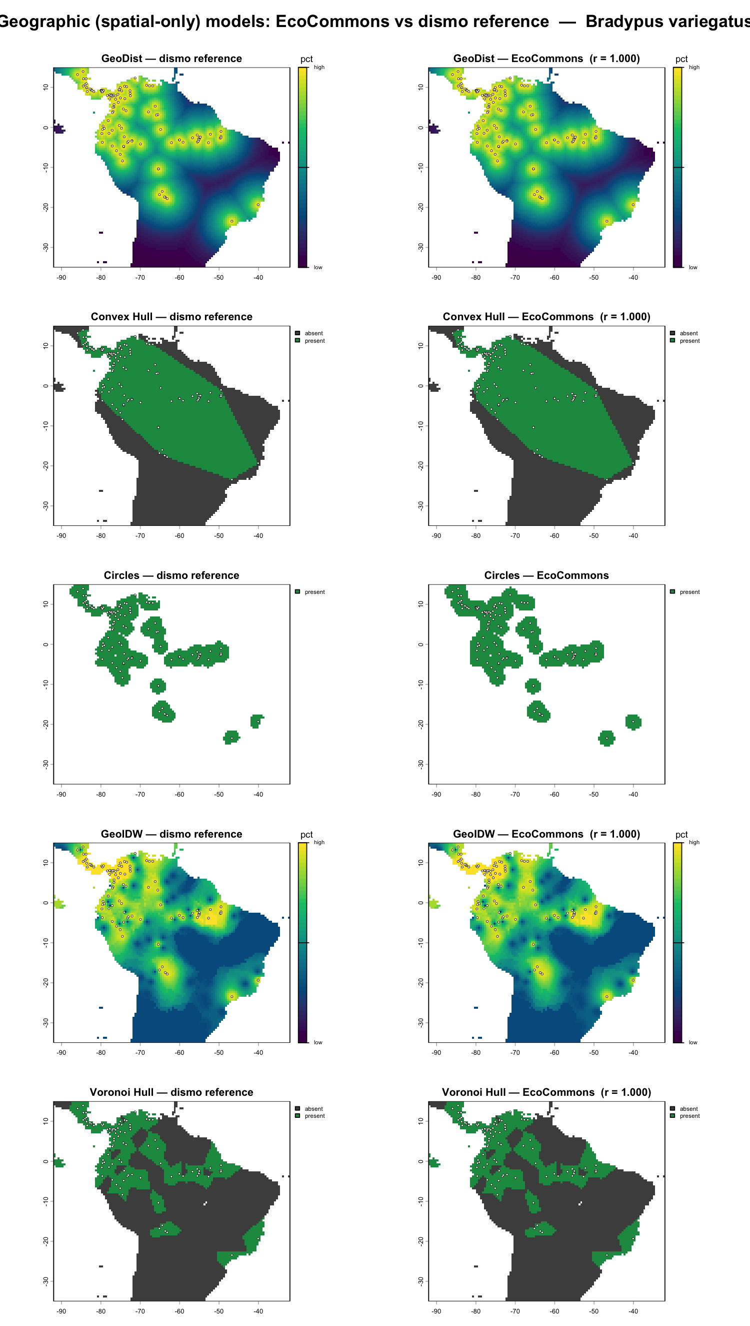
Each row is one geographic model, dismo reference (left) vs the EcoCommons projection (right), over the Bradypus variegatus* range; white points are the occurrence records the model was fitted on. Continuous models (GeoDist, GeoIDW) use a percentile colour stretch; binary models (Convex Hull, Circles, Voronoi Hull) show presence (green) vs absence (grey). For every model the two columns are visually indistinguishable — GeoDist, Convex Hull, GeoIDW and Voronoi Hull agree at Pearson r = 1.000, and Circles reproduces the reference presence footprint exactly.*

Prediction maps

Single-species benchmark predictions

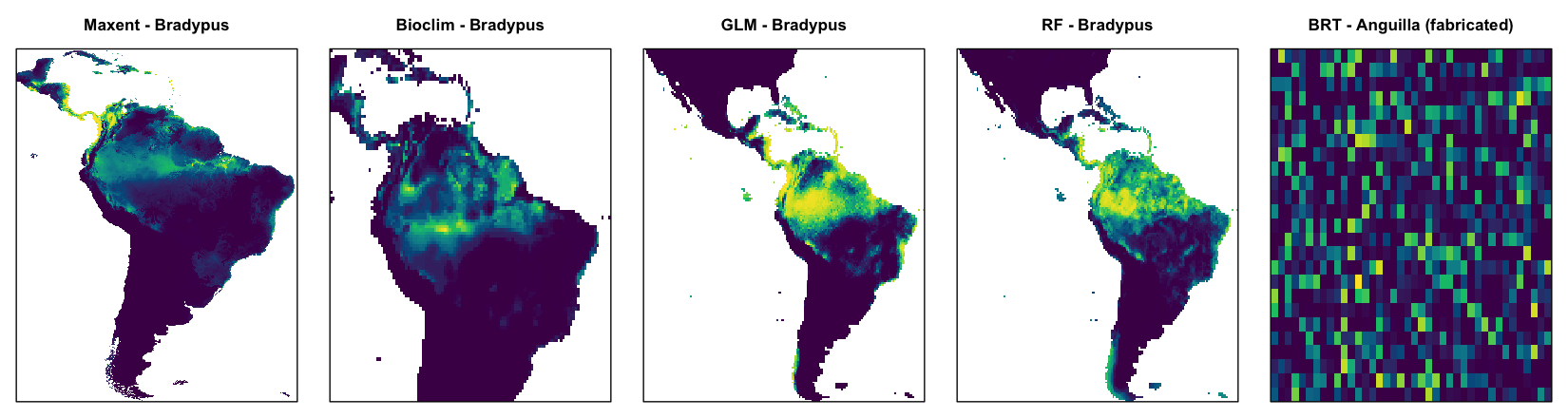
Bradypus (South America): Maxent, Bioclim, GLM, RF. Anguilla BRT is on a fabricated one-cell-per-site grid (scattered pixels), so its “map” is not geographically meaningful — only its per-site predictions are.

nsw14 (Valavi) — continuous surface, published points & agreement

The clearest check places each algorithm in one row across three columns: (1) our continuous re-fit of Valavi’s config predicted across the whole NSW grid, (2) Valavi et al. (2021)’s own published point predictions (Models_prediction/*.csv) at the 702 evaluation sites, and (3) the site-level agreement — our raster value at each site (y) against Valavi’s published value (x), with the 1:1 line and per-model Pearson r. Columns 1–2 share the same 0–1 suitability scale; red rings mark observed presences.

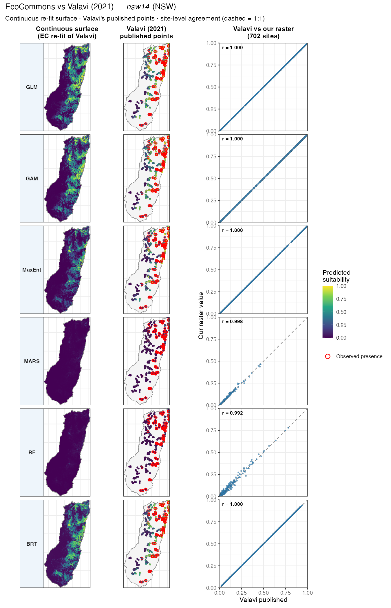
For every algorithm the published points fall on our continuous surface — same eastern escarpment / north-east coast hotspot, same magnitude — and the agreement column makes it quantitative: GLM/GAM/MaxEnt/BRT collapse onto the 1:1 line (r = 1.000), MARS 0.998, RF 0.992 (small stochastic scatter). The points are Valavi’s actual published values (disPa coordinates over the NSW border), not our reproduction, so this comparison is independent of our package-version environment. This is the per-model view of the 702-site table below.

These maps reproduce Valavi’s published predictions. Extracting each raster band at Valavi’s 702 evaluation sites and correlating with the original Models_prediction/*.csv:

model	Pearson	Spearman	match
GLM	1.0000	1.0000	exact
GAM	1.0000	1.0000	exact
MaxEnt	1.0000	1.0000	exact
BRT	1.0000	1.0000	exact
MARS	0.9976	0.9980	near-perfect
RF	0.9922	0.9296	high (RF vote-fraction ties lower Spearman)

This works because disEnv — the environmental values Valavi predicted their points on — is itself sampled from these NSW rasters, so the raster value at each site is the value Valavi used. GLM, GAM, MaxEnt and BRT reproduce it exactly; MARS/RF show only small stochastic / version scatter (RF’s vote-fraction ties lower its Spearman). The agreement column of the figure above is the per-model, Pearson view of this table.

Agreement analysis

EcoCommons vs benchmark — every test

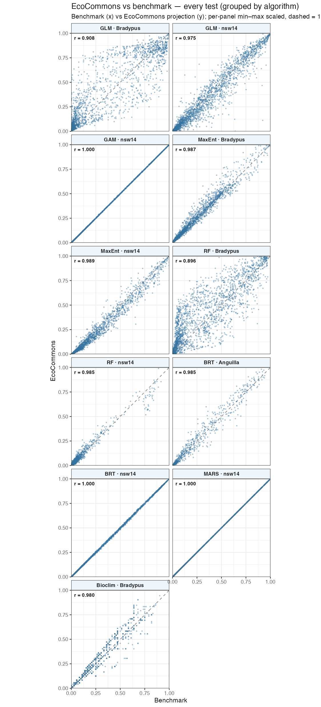
Single-species tests (Bradypus / Anguilla) and nsw14 vs Valavi, grouped by algorithm. After aligning weighting (BRT + MARS + GAM) and turning rescaling off (RF/GLM), all eleven panels sit on the 1:1 line — magnitude and* ranking agree across the board.*

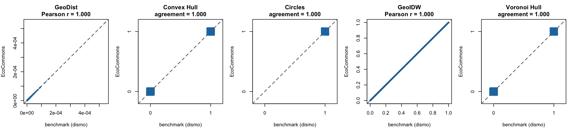
The five geographic (spatial-only) models (tests 12–16), EcoCommons projection (y) vs the dismo reference on identical inputs (x). Continuous models (GeoDist, GeoIDW) collapse onto the 1:1 line (Pearson r = 1.000); the binary models (Convex Hull, Circles, Voronoi Hull) match cell-for-cell (agreement = 1.000, jittered so the 0/0 and 1/1 clusters are visible). Circles is shown after its fix. Every geographic model is an exact match to its dismo reference.

Reproducibility & benchmark provenance

The single most important thing to understand about these nsw14 benchmarks is what they are a reference to — because it determines when they must be regenerated and what “still matching Valavi” actually means.

Two different reference points

There are two distinct notions of “matching a reference”, and they behave very differently:

	Independent reimplementation (what the .tif benchmarks are)	Published paper numbers (Valavi’s Models_prediction/*.csv)
Produced by	generate_nsw14_valavi_benchmarks.R — Valavi’s exact configs re-run through the algorithm’s own R package (gam, randomForest, earth, dismo::maxent, dismo::gbm.step)	Valavi et al. (2021), fixed external artifact
What the test checks	Implementation fidelity — does EcoCommons wire up the algorithm the same way an independent implementation does?	Literature agreement — do we reproduce the actual published predictions?
Metric used here	Pearson on absolute suitability (the agreement tables above)	Pearson/Spearman at the 702 evaluation sites (the “reproduce Valavi’s published predictions” table above)
Sensitive to package version?	Cancels out — see below	Yes — this is the real anchor to the paper

The .tif benchmarks are not frozen EcoCommons snapshots (they come from different engines) and not Valavi’s literal published rasters either. They are a faithful re-run of Valavi’s recipe. So “matching the paper” via these benchmarks means “matching a faithful reproduction of Valavi’s config”, not bit-matching the 2021 output.

What changes the final benchmark

The absolute suitability values written into each benchmark .tif depend on the software environment they were generated in — not just the algorithm and config. In order of impact:

1. Package version drift. Tree-ensemble learners are the main offender: gbm (BRT) absolute predicted probabilities shift across gbm versions / platforms. randomForest, earth, gam, maxent.jar are far more stable. This is the reproducibility issue that forced the BRT benchmark to be regenerated inside the CI container rather than frozen from a dev machine (newer gbm on macOS drifts on Pearson in CI).
2. The R version and compiler toolchain (numerical libraries, BLAS).
3. Config / weighting changes — e.g. background down-weighting, normalisation, hyper-parameters. BRT down-weighting is now applied through the supported site_weight_scheme = "downweight" option in the nsw14_brt spec (no longer a test-only mock), so EcoCommons matches Valavi’s config directly.
4. The training-point construction — dedup one-per-cell, complete-cases filtering — which is deliberately matched to EcoCommons’ filter.raster.

Because of (1)–(2), benchmarks must be regenerated in the pinned CI container (ec-rpkg-ci-test-env), never on a local dev machine. Locally, R is not renv-activated, so a laptop pulls whatever package versions it happens to have — reintroducing exactly the drift the CI-native benchmark exists to avoid.

Why regenerating in the same environment is safe

When a benchmark is regenerated in a bumped environment, both the benchmark and EcoCommons run through the same new engine (for BRT, the same new gbm). Their absolute values shift together, so their Pearson agreement is preserved. That is precisely why regenerating-in-CI works: it cancels version drift on both sides.

The blind spot: because the two sides move together, a genuine engine change could move both the benchmark and EcoCommons away from Valavi’s 2021 numbers while they still agree with each other. The guard against silently re-baselining away from the paper is twofold:

• Rank-drift check (in the generator). write_bench() reports the Spearman correlation between each newly generated prediction and the currently committed .tif, and warns if it drops below 0.98. Benign scale drift (a new gbm) leaves rank order intact (Spearman ≈ 1); a low Spearman means the science moved, not just the scale — investigate before committing.
• Literature anchor. The “reproduce Valavi’s published predictions” table (702-site Pearson/Spearman vs the original CSVs) is the check that actually ties us to the paper, and it is version-robust because it is rank-friendly.

Rule of thumb: benchmark-generation environment == test-execution environment == the pinned container image. Whenever that pin moves (a package patch or a base-image rebuild), regenerate the affected .tif benchmarks in the new environment and commit them alongside the version bump — after confirming the rank-drift guard stays green.

Reproducibility environment — pinned package versions

These are the versions the benchmarks and agreement tests are pinned to, from renv-main.lock (== the deployed base image ec-base-r4.2 / CI test image ec-rpkg-ci-test-env). The base image is rebuilt only via a manual pipeline (BUILD_BASE=1); renv is not auto-activated, so this lock governs the container, not ad-hoc local runs.

R 4.2.2 · CRAN snapshot https://cloud.r-project.org

Package	Version	Role in the agreement suite
biomod2	4.2-2	EcoCommons GLM / RF / MARS engine (wraps the learners below)
dismo	1.3-9	EcoCommons BRT (gbm.step), MaxEnt (maxent.jar), Bioclim
gbm	2.1.8.1	BRT learner — version-sensitive; drives CI-native regeneration
randomForest	4.7-1.1	RF learner + Valavi RF benchmark
earth	5.3.2	MARS learner + Valavi MARS benchmark
terra	1.7-3	Raster I/O, benchmark grid, cell dedup
raster	3.6-14	dismo/raster-style stacks for geographic models
sf	1.0-9	Vector geometry / constraint regions
caret	6.0-93	Valavi’s original Appendix S2 MARS tuning (continuous maps)
testthat	3.1.6	Test runner (pinned; avoid newer-only features in CI)

Generation-only, not pinned in the lock: gam::step.Gam (GLM benchmark), mgcv::gam (GAM benchmark) and rJava (MaxEnt/JVM) are installed on top of the base image rather than via renv, so they take whatever the CI image provides at generation time. gam / mgcv are used only to build the GLM / GAM .tif benchmarks, not by the EcoCommons runtime.

Cross–R-version reproducibility: eight biomod2 learners across R 3.4.1 → 4.5.0

All eight HSDM learners are guarded by scientific-agreement tests (the Vulpes vulpes rows above). Getting there began as a controlled study of what actually breaks reproducibility: we reproduced each one exactly as taught in Guisan, Thuiller & Zimmermann’s Habitat Suitability and Distribution Models (2017; the public hsdm companion code), then re-ran it under the book’s original 2017 software and under a current stack, and diffed the predictions cell-by-cell. The first four (SRE · FDA · ANN · GBM) came first; the deterministic batch (GLM · GAM · MARS · CTA) was added later, each under period-correct 2017 packages (stats base, mgcv 1.8-17, earth 4.5.1, rpart 4.1-11).

Setup. Species Vulpes vulpes (red fox); the book’s mammals_and_bioclim_table (8,542 global grid cells, 4,203 presences / 4,339 absences at 1.5°); four predictors bio3, bio7, bio11, bio12. Model calls are the book’s verbatim configurations (biomod2::sre; mda::fda(method = mars); nnet, size 6 / decay 0.001; gbm, bernoulli / 10 000 trees / depth 3 / shrinkage 0.01 / 10-fold CV; glm logit; mgcv::gam default s(); earth degree 1 logit; rpart method="class", xval 10), same set.seed(555) where stochastic. The “old” environment is a pinned Docker image (rocker/r-ver:3.4.1); the “new” one is current CRAN.

Component	Old environment (Docker)	Current environment
R	3.4.1 (2017-06-30)	4.5.0 (2025)
SRE	biomod2 3.3-7 sre() verbatim	biomod2 4.2-2 bm_SRE
FDA	mda 0.4-9	mda 0.5-5
ANN	nnet 7.3-12	nnet 7.3-20
GBM	gbm 2.1.3	gbm 2.2.3
GLM	stats::glm (base 3.4.1)	stats::glm (base 4.5.0)
GAM	mgcv 1.8-17	mgcv 1.9-4
MARS	earth 4.5.1	earth 5.3.5
CTA	rpart 4.1-11	rpart 4.1-24

Result — reproducibility tracks determinism.

Algorithm	Nature	Cross-version agreement	Verdict
SRE	deterministic envelope	100% cells identical	exact
GLM	deterministic (IRLS)	Pearson 1.0000 (max Δ 6×10⁻¹⁵)	exact
CTA	deterministic tree	8542/8542 cells identical	exact
MARS	deterministic (earth)	Pearson 1.0000 (max Δ 1×10⁻¹³)	exact
FDA	deterministic (MARS)	Pearson 1.0000	exact
GAM	deterministic (penalised)	Pearson 0.99995 (max Δ 0.05)	tiny drift (mgcv version)
ANN — single fit	stochastic (random init)	Pearson 0.945	diverges
ANN — 15× ensemble	stochastic, averaged	Pearson 0.997	largely fixed
GBM	stochastic (bagging + CV)	Pearson 0.9997	near-identical

The deterministic batch confirms the pattern — with one instructive exception. GLM, MARS and CTA are bit-identical across the eight-year gap (differences at the 10⁻¹³–10⁻¹⁵ floating-point floor; CTA reproduces every one of 8,542 cells exactly). GAM is the outlier: still deterministic, but it drifted by up to 0.05 (Pearson 0.99995) — not from randomness, but because mgcv’s smoothing changed between 1.8-17 (2017) and 1.9-4 (2025). That is the key distinction from ANN: CTA/GLM/MARS reproduce because the algorithm is fixed; GAM’s small drift is a deliberate implementation change, not the compiled-environment noise that makes a single ANN diverge.

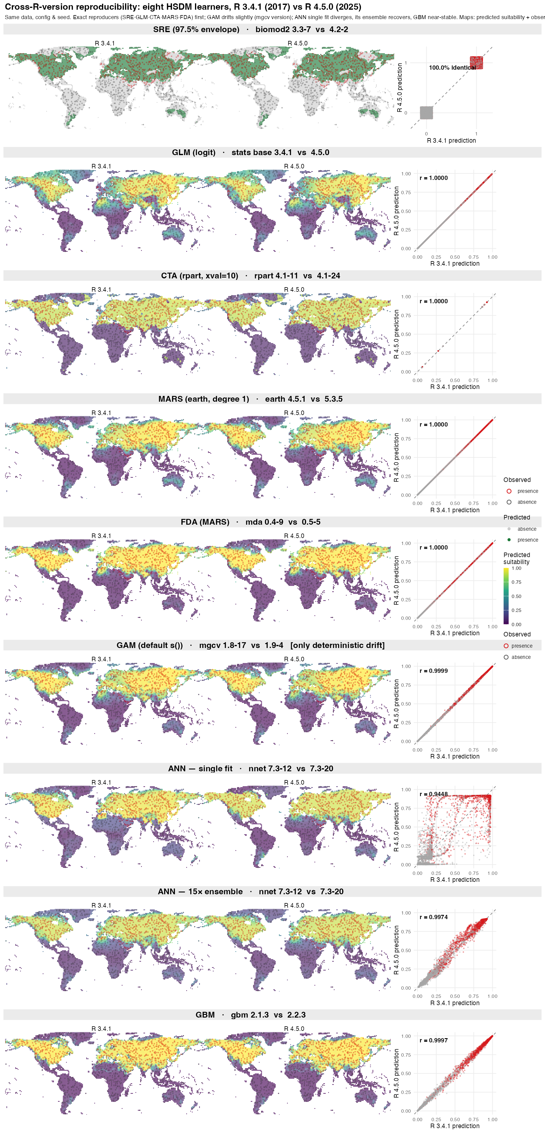
All eight learners (nine rows — ANN appears as both a single fit and a 15× ensemble), ordered by the determinism story. Each row is one model: predicted suitability under R 3.4.1 (left) vs R 4.5.0 (middle) — sharing a suitability scale, with observed occurrences as rings (red = presence, grey = absence) — and the agreement scatter (right): old (x) vs new (y), dashed 1:1 line, Pearson r, dots coloured by observed status. SRE, GLM, CTA, MARS and FDA reproduce to the bit (tight diagonals); GAM drifts only slightly (mgcv version change); a single ANN drifts into a “leaf”-shaped cloud; averaging 15 ANN fits pulls it back onto the diagonal; GBM barely moves. Styling matches the paired figures above.

Methods — metrics for reproduction performance

Every agreement test runs a real EcoCommons projection and compares it, cell by cell over the prediction grid, against an independent benchmark (for the HSDM suite, our verbatim reproduction of the book). We score the two rasters with two complementary correlation metrics, and read the shape of their scatter to diagnose how they (dis)agree.

Two metrics

• Pearson correlation — agreement on the absolute predicted values. It reaches 1.0 only if the two surfaces are related by a straight line, so it penalises any difference in scale or probability calibration. This is the strict headline metric, used where both engines are on the same 0–1 scale (as on the balanced HSDM Vulpes data).
• Spearman rank correlation — agreement on the ordering of cells. It reaches 1.0 whenever the two surfaces rank every cell the same way, regardless of the value scale; it is invariant to any monotonic transform (rescaling, a different sigmoid/posterior calibration, etc.).

Why both. For an SDM the ecologically meaningful quantity is usually the ranking of suitability — which places are more suitable, where a threshold falls — not the absolute probability scale. So a high Spearman with a lower Pearson means “same science, different scale”: a benign recalibration, not a scientific disagreement. We report Pearson where the scales match and lean on Spearman when a monotonic scale difference would otherwise understate an exact match.

Reading the agreement scatter

Plotting benchmark (x) against EcoCommons (y) makes the kind of agreement visible:

Scatter shape	Meaning	Example
Straight line on the 1:1 diagonal	exact agreement (Pearson ≈ Spearman ≈ 1)	SRE
Clean S-curve, no scatter	deterministic monotonic rescaling — identical ranking (Spearman = 1), slightly different value scale; benign	FDA (r_s = 1.000, r = 0.999)
Lens / “almond” cloud	stochastic disagreement — genuine run-to-run noise, widest in the uncertain mid-range (~0.5) and pinched where predictions saturate (0/1), tracking p(1 − p)	GBM (thin), ANN (fat)

The S-curve and the almond are two faces of the same sigmoid output transform: the S is its noiseless skeleton (a pure rescaling), the almond is that skeleton smeared by stochastic noise. A fat almond means large noise (a single ANN’s random weight initialisation → different local minima); GBM’s per-tree bagging almond is by contrast negligible — averaged over 10,000 trees, almost nothing survives — so once its config is matched GBM’s scatter is essentially a straight line.

Deterministic vs stochastic learners

This taxonomy sets the achievable ceiling:

• Deterministic — SRE (quantile envelope) and FDA (MARS) compute a single fixed answer, so any correct implementation reproduces them to Pearson/Spearman ≈ 1 (FDA’s tiny S is a rank-preserving wrapper hairline, not a disagreement).
• Stochastic — GBM (bagging) and ANN (random weight init) carry irreducible noise, but they land in very different places. GBM reproduces to ~0.999 with a single fit once its config is matched: its per-tree bagging noise is already averaged away by the 10,000-tree ensemble, so almost nothing survives. (Its earlier 0.955 was a config mismatch — the benchmark used the book’s GBM settings while EcoCommons fell back to biomod2’s defaults — not bagging noise; pinning the config fixes it.) A single ANN fit is the opposite: it does no internal averaging, so it lands in a different local minimum every time and reproduces only to ~0.81 — which is why we test ANN as a 50× ensemble (→ 0.996). The general rule: averaging turns a non-reproducible stochastic learner into a reproducible one — GBM does it internally (10k trees), we do it explicitly for ANN (50 nets).

Per-algorithm pass thresholds reflect this: 0.99 for SRE, FDA and GBM, and 0.95 for the ANN ensemble.

EcoCommons agreement on the HSDM data (SRE · FDA · ANN · GBM)

The cross-version work above validates the reference implementation. The final step closes the loop: does EcoCommons itself reproduce that reference? We converted the book’s Vulpes vulpes data into EcoCommons input fixtures (4,203 presences / 4,339 absences on the 1.5° global grid, with bio3/bio7/bio11/bio12), ran EcoCommons’ own SRE / FDA / ANN / GBM, and scored each projection against our verbatim reproduction of Guisan, Thuiller & Zimmermann (2017) — i.e. the benchmark is the projection we made, not a frozen EcoCommons snapshot. These are now testthat agreement tests in the EcoCommons R package (test-sdm_projection_agreement.R, hsdm_* specs).

Algorithm	Engine	Nature	Pearson	Spearman	Result
SRE	biomod2 (envelope)	deterministic	1.000	1.000	✅ exact
FDA	mda (MARS)	deterministic	0.999	1.000	✅ exact
GBM	gbm	stochastic (bagging)	0.999	0.999	✅ exact
ANN	nnet	stochastic — 50× ensemble †	0.996	0.993	✅ reproduced

† ANN is changed from the book — and why

The book fits a single ANN. But a single neural network is not a reproducible object: its non-convex training lands in an arbitrary local minimum set by the random starting weights, and across seeds the model quality swings wildly (AUC 0.73–0.97 on this data). Two independent implementations therefore never match — the book’s ANN and EcoCommons’ ANN agree only at Pearson ≈ 0.81, and neither is even reproducible run-to-run.

So for ANN we deliberately change the configuration to an ensemble: fit 50 networks, each on a different random 80/20 split, and average them (EcoCommons’ native nb_run_eval = 50). Averaging converges to the stable expected prediction — a well-defined, reproducible target. The payoff: EcoCommons’ 50-net ensemble reproduces our 50-net ensemble at Pearson 0.996, and the EcoCommons ensemble is itself reproducible run-to-run at 0.999 (a single fit was neither). This is a strictly better model than the book’s single fit, and it moves ANN from “the fragile outlier” into the reproducible column. You cannot reproduce one coin flip; you can reproduce the average of 50.

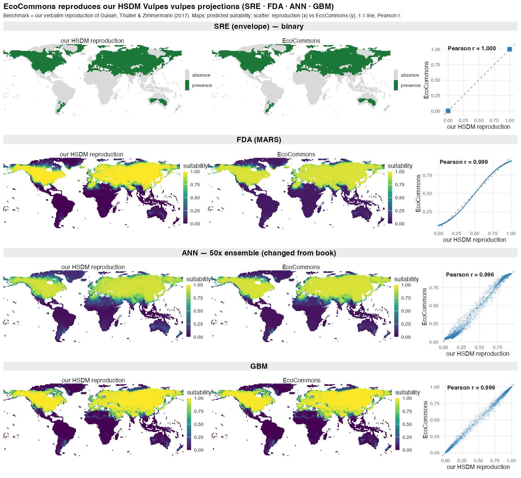
Each row is one algorithm: our HSDM reproduction (left) vs the EcoCommons projection (middle), over the global Vulpes vulpes range, and the site-level agreement (right) — our value at each cell (x) against EcoCommons’ (y), with the 1:1 line and Pearson r. All four scatters collapse onto the 1:1 line and the map columns are visually indistinguishable. On the balanced Vulpes presence/absence with the book’s verbatim configuration both engines sit on the same 0–1 scale, so Pearson (not just rank) is high. ANN is the 50× ensemble (changed from the book — see the note above): a single ANN fit would open into a noisy cloud (Pearson ≈ 0.81, an arbitrary local minimum), but averaging 50 fits converges to a stable, reproducible surface that EcoCommons reproduces to Pearson 0.996.

The deterministic batch (GLM · GAM · MARS · CTA)

The four regression / classification learners the book teaches on the fox — GLM (§10.2), GAM (§10.3), MARS (§10.4) and CTA (§11.2) — have no randomness in the fit, so the book’s bare call is an exact reproducible target. Each reproduces to Pearson 1.000 once the JSON pins biomod2 to the book’s configuration. (The one snag was MARS: biomod2 encodes interactions through the model formula, not earth’s own degree= argument, so its exposed MARS matches the book’s degree-1 Mars_int1, not the degree-2 Mars_int2.)

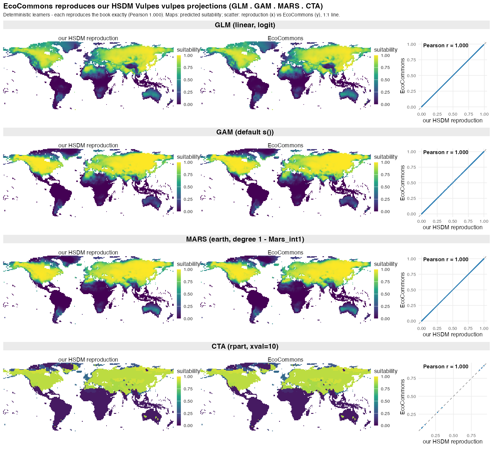
Same layout as above, for the deterministic batch. GLM/GAM/MARS produce smooth suitability surfaces; CTA is a classification tree, so its map is piecewise-constant (a few discrete bands) and its scatter is a staircase of point-clusters — both sitting exactly on the 1:1 line. All four collapse to Pearson 1.000 (CTA scored on Spearman rank, as its ties make Pearson brittle): EcoCommons reproduces the book’s projections cell-for-cell.

Why CTA clusters — the tree and its response curves

CTA’s stepped map and clustered scatter are not an artifact: a classification tree partitions the predictors into a finite set of leaf nodes, and every cell in a leaf gets the same predicted probability. This tree has 8 leaves, so across all 8,542 cells CTA emits only 8 distinct values (vs ~7,000–8,400 for GLM/GAM/MARS) — which is exactly why its scatter collapses to an 8-point staircase and why it reproduces cell-for-cell across R versions.

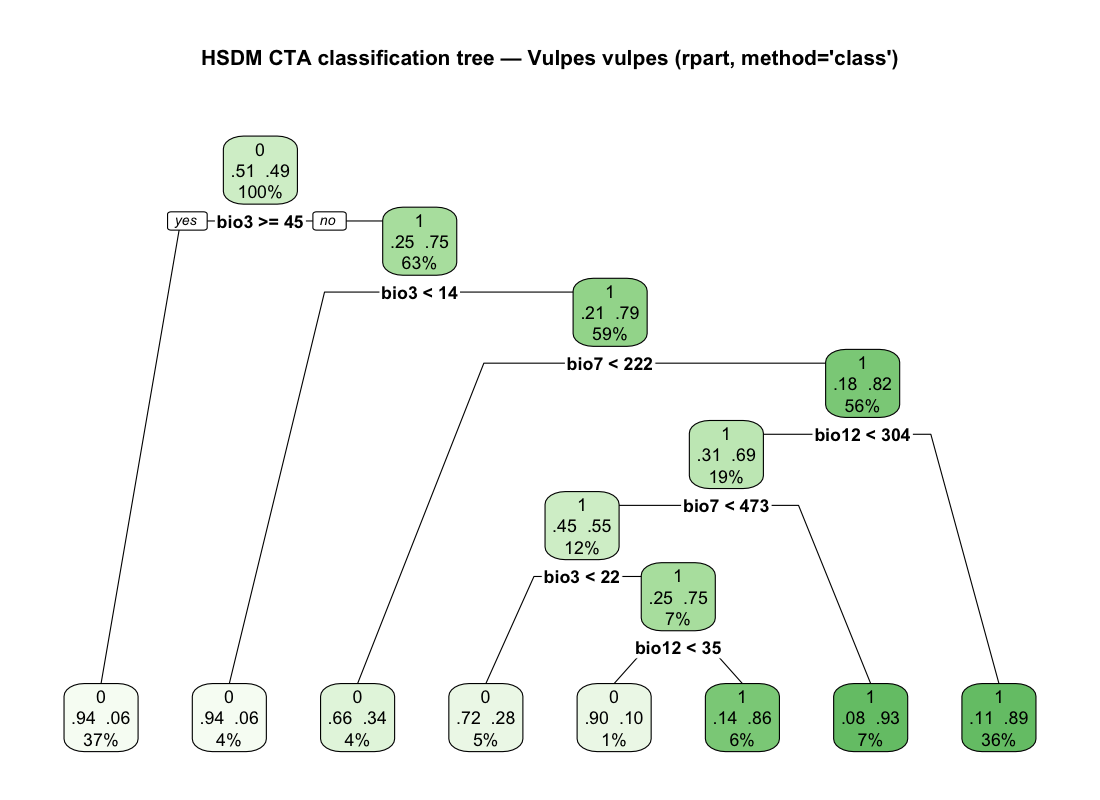
The fitted rpart tree (book Fig 11.1 equivalent). Each box gives the predicted class, the (absence, presence) probabilities, and the share of data in the node. The root split bio3 ≥ 45 (isothermality) separates tropical cells (→ absence) from the rest; deeper splits on bio3, bio7 and bio12 carve out the temperate northern-hemisphere fox range. The 8 leaves are the 8 distinct prediction values.

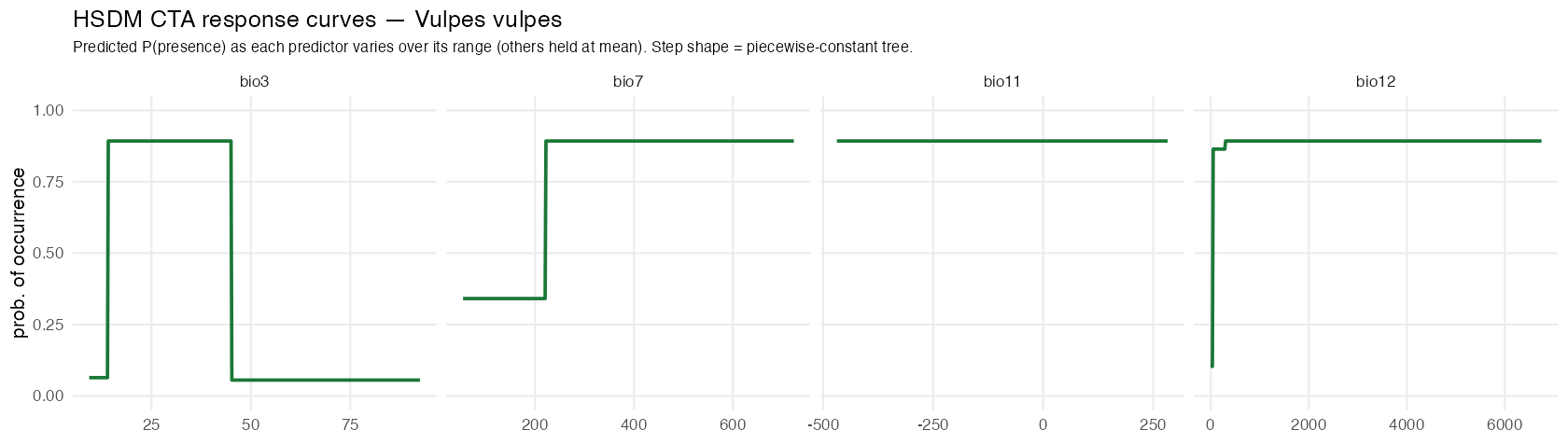
Response curves (book Fig 11.3 equivalent): predicted P(presence) as each predictor sweeps its range with the others held at their mean. The curves are step functions whose jumps sit at the tree’s split thresholds — a “window” of suitability in bio3 (~14–45), one step in bio7, a sharp step at low bio12, and a flat bio11 (no split on that variable is reached along this path).

References

• Booth, T.H., Nix, H.A., Busby, J.R. & Hutchinson, M.F. (2014). BIOCLIM: the first species distribution modelling package, its early applications and relevance to most current MaxEnt studies. Diversity and Distributions 20: 1–9.
• Guisan, A., Thuiller, W. & Zimmermann, N.E. (2017). Habitat Suitability and Distribution Models: With Applications in R. Cambridge University Press. (SRE / FDA / ANN / GBM reproduction and the cross–R-version experiment; companion hsdm code.)
• Breiman, L. (2001). Random forests. Machine Learning 45: 5–32.
• Elith, J., Leathwick, J.R. & Hastie, T. (2008). A working guide to boosted regression trees. Journal of Animal Ecology 77: 802–813.
• Elith, J., Graham, C.H., Valavi, R., Abegg, M., Bruce, C., Ford, A., Guisan, A., Hijmans, R.J., Huettmann, F., Lohmann, L.G., Loiselle, B.A., Moritz, C., Overton, J.McC., Peterson, A.T., Phillips, S., Richardson, K., Williams, S., Wiser, S.K., Wohlgemuth, T. & Zimmermann, N.E. (2020). Presence-only and presence-absence data for comparing species distribution modeling methods. Biodiversity Informatics 15: 69–80. (NCEAS data; distributed via the disdat R package and OSF project kwc4v.)
• Friedman, J.H. (1991). Multivariate adaptive regression splines. The Annals of Statistics 19: 1–67.
• Hastie, T.J. & Tibshirani, R.J. (1990). Generalized Additive Models. Chapman & Hall. (gam::step.Gam stepwise selection.)
• Hijmans, R.J., Phillips, S., Leathwick, J. & Elith, J. dismo: Species Distribution Modeling. R package. (gbm.step, maxent, bioclim.)
• Hijmans, R.J. & Elith, J. Species distribution modeling with R. (The dismo package vignette; Chapter 13 “Geographic models” — geoDist, convHull, circles, geoIDW, voronoiHull.)
• McCullagh, P. & Nelder, J.A. (1989). Generalized Linear Models, 2nd edn. Chapman & Hall.
• Nix, H.A. (1986). A biogeographic analysis of Australian elapid snakes. In: Atlas of Elapid Snakes of Australia (ed. R. Longmore), pp. 4–15. Australian Government Publishing Service.
• Phillips, S.J., Anderson, R.P. & Schapire, R.E. (2006). Maximum entropy modeling of species geographic distributions. Ecological Modelling 190: 231–259.
• Phillips, S.J. & Dudík, M. (2008). Modeling of species distributions with Maxent: new extensions and a comprehensive evaluation. Ecography 31: 161–175.
• Thuiller, W., Lafourcade, B., Engler, R. & Araújo, M.B. (2009). BIOMOD – a platform for ensemble forecasting of species distributions. Ecography 32: 369–373. (biomod2 R package.)
• Valavi, R., Guillera-Arroita, G., Lahoz-Monfort, J.J. & Elith, J. (2021). Predictive performance of presence-only species distribution models: a benchmark study with reproducible code. Ecological Monographs 92(1): e01486. (Appendix S1/S2 configurations; Models_prediction per-species outputs.)
• Wood, S.N. (2017). Generalized Additive Models: An Introduction with R, 2nd edn. Chapman & Hall/CRC. (mgcv package; GAM benchmark engine.)