Calculating and Visualising Species Richness and Shannon Diversity for Ecological Survey Data

Author details: Dr Ryan Newis

Editor details: Xiang Zhao

Contact details: support@ecocommons.org.au

Copyright statement: This script is the product of the EcoCommons platform. Please refer to the EcoCommons website for more details: https://www.ecocommons.org.au/

Date: June 2025

Script and Data Information

This notebook, developed by the EcoCommons team, showcases how to calculate, analyse and compare species richness and species diversity (Shannon) across different landscapes and sites for bird survey data. This method can be applied to other animals, plants or biological communities that use a similar surveying method.

Pale-headed Rosella - Platycercus adscitus: Photographer: Chris Murray

Introduction

Understanding how to calculate species richness and Shannon diversity is essential for assessing baseline biodiversity in ecological studies (Hill 1973; Gotelli and Colwell 2001; Chao and Chiu 2016). These metrics provide valuable insights into both the number of species present (richness) and the evenness of species distribution (Shannon diversity), helping ecologists monitor ecosystem health, detect changes over time, and inform conservation and management decisions.

Key Concepts

K.1 Species richness

Species richness is a fundamental measure of biodiversity, reflecting the total number of species within a defined area or ecological community. It serves as a key indicator of habitat complexity and ecosystem health, providing a baseline for understanding patterns of species distribution and the potential effects of environmental change (Gotelli & Colwell 2001; Gotelli et al. 2009).

K.2 Shannon diversity

Shannon diversity (also known as the Shannon-Wiener Index) integrates both species richness and the relative abundance of each species within a community. It provides a quantitative measure of biodiversity that accounts for species evenness, offering deeper insights into community structure and the dominance or rarity of species across ecological gradients (Shannon 1948; Hill 1973; Magurran 2004).

K.3 Landscape comparisons in ecology

Landscape-level comparisons allow ecologists to assess how species assemblages and biodiversity metrics vary across different environmental contexts. By comparing landscapes — such as forests and urban areas — researchers can identify the influence of habitat type, land-use change, and human disturbance on ecological communities. These comparisons are critical for understanding patterns of biodiversity loss, informing conservation priorities, and guiding land management strategies aimed at maintaining ecosystem integrity (Turner 1989; Turner 2001; Fahrig 2003).

Objectives

Learn how to prepare datasets for species richness and Shannon diversity calculations.
Learn how to calculate, statistically compare, and visualise species richness.
Learn how to calculate, statistically compare, and visualise Shannon diversity.

Workflow Overview

Step 1: Set-up - Install and load required R packages (libraries)
Step 2: Loading and preparing data
Step 3: Species richness calculations, comparisons, and visualisations
Step 4: Shannon diversity calculations, comparisons, and visualisations

In the near future, this material may form part of comprehensive support materials available to EcoCommons users. If you have any corrections or suggestions to improve the efficiency, please contact the EcoCommons team.

Step 1: Set-up R environment and packages

Some housekeeping before we start. This process might take some time as multiple packages may need to be installed.

1.1 Set the working directory and create a folder for data.

Save the Quarto Markdown file (.QMD) to a folder of your choice, and then set the path to your folder as your working directory.

# Set the workspace to the current working directory
#setwd('path_to_your_folder')
#setwd('/Users/ryannewis/Documents/GitHub/Repositories/Richness_diversity/notebooks')

Now your local working drive is set.

1.2 Install and load required packages

Install and load R packages and libraries.

# Install and load required packages (if not already installed)
required_packages <- c(
  "ggplot2",
  "vegan",
  "tidyr",
  "dplyr",
  "multcompView",
  "lme4",
  "lmerTest",
  "emmeans",
  "stringr"
)

# Identify missing packages
missing_packages <- required_packages[!(required_packages %in% installed.packages()[,"Package"])]
# Install only missing packages

if (length(missing_packages) > 0) {
  install.packages(missing_packages)
}
# Load all required packages
lapply(required_packages, library, character.only = TRUE)

[[1]]
[1] "ggplot2"   "stats"     "graphics"  "grDevices" "utils"     "datasets" 
[7] "methods"   "base"     

[[2]]
 [1] "vegan"     "permute"   "ggplot2"   "stats"     "graphics"  "grDevices"
 [7] "utils"     "datasets"  "methods"   "base"     

[[3]]
 [1] "tidyr"     "vegan"     "permute"   "ggplot2"   "stats"     "graphics" 
 [7] "grDevices" "utils"     "datasets"  "methods"   "base"     

[[4]]
 [1] "dplyr"     "tidyr"     "vegan"     "permute"   "ggplot2"   "stats"    
 [7] "graphics"  "grDevices" "utils"     "datasets"  "methods"   "base"     

[[5]]
 [1] "multcompView" "dplyr"        "tidyr"        "vegan"        "permute"     
 [6] "ggplot2"      "stats"        "graphics"     "grDevices"    "utils"       
[11] "datasets"     "methods"      "base"        

[[6]]
 [1] "lme4"         "Matrix"       "multcompView" "dplyr"        "tidyr"       
 [6] "vegan"        "permute"      "ggplot2"      "stats"        "graphics"    
[11] "grDevices"    "utils"        "datasets"     "methods"      "base"        

[[7]]
 [1] "lmerTest"     "lme4"         "Matrix"       "multcompView" "dplyr"       
 [6] "tidyr"        "vegan"        "permute"      "ggplot2"      "stats"       
[11] "graphics"     "grDevices"    "utils"        "datasets"     "methods"     
[16] "base"        

[[8]]
 [1] "emmeans"      "lmerTest"     "lme4"         "Matrix"       "multcompView"
 [6] "dplyr"        "tidyr"        "vegan"        "permute"      "ggplot2"     
[11] "stats"        "graphics"     "grDevices"    "utils"        "datasets"    
[16] "methods"      "base"        

[[9]]
 [1] "stringr"      "emmeans"      "lmerTest"     "lme4"         "Matrix"      
 [6] "multcompView" "dplyr"        "tidyr"        "vegan"        "permute"     
[11] "ggplot2"      "stats"        "graphics"     "grDevices"    "utils"       
[16] "datasets"     "methods"      "base"

Now all required packages have been installed and loaded.

Step 2: Downloading and preparing data

If you’re using your own bird survey data, here’s how to prepare it. The analysis in this notebook expects your data to initially be structured as a “long format” CSV file (see Table 1 for example.).

Table 1. Expected data structure (long format): Each row should represent one observation of species abundance at a specific study site and time, e.g. :

Site	Time	Landscape	Species	Abundance
Forest_Site1	January	Forest	Bird A	23
Forest_Site2	January	Forest	Bird B	11
Urban_Site1	January	Urban	Bird A	5
Urban_Site2	January	Urban	Bird B	9

Column names must be exactly: “Site”, “Time”, “Landscape”, “Species”, “Abundance” to work directly with the code in this notebook. This notebook will automatically convert the long-format data to wide format when needed (e.g., for diversity index calculations).

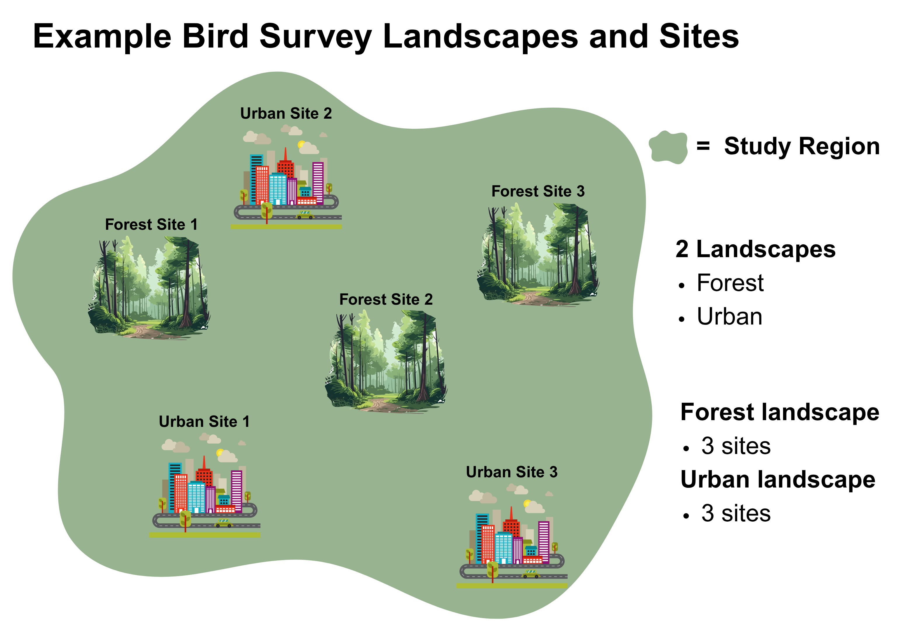
The image below depicts the study design for the example bird survey used in this notebook workflow. The design incorporates and compares 2 contrasting landscapes: Forest and Urban. Each landscape has 3 sites in which bird surveys were conducted.

Now we will load in the CSV data file (in long format) and check the data structure.

Replace “example_birdsurvey_data.csv” with the actual path to your file when doing analysis of your own data

# Load example dataset from EcoCommons GitHub
your_data <- read.csv("https://raw.githubusercontent.com/EcoCommonsAustralia/notebooks/Richness_diversity/notebooks/example_birdsurvey_data.csv")

#If you want to download a copy of the dataset to your local computer use the code below. Today we will just be calling the dataset which will remain in in the R environment for the session.
# download.file(
#   "https://raw.githubusercontent.com/EcoCommonsAustralia/notebooks/Richness_diversity/notebooks/example_birdsurvey_data.csv")

#Then you would load the data directly from your local drive
#your_data <- read.csv("example_birdsurvey_data.csv", stringsAsFactors = FALSE)

#Alternatively can save this dataset locally by running this line at any time
#write.csv(your_data, "example_birdsurvey_data.csv", row.names = FALSE)


# Check the data structure
str(your_data)

'data.frame':   473 obs. of  6 variables:
 $ Site     : chr  "Forest_Site1" "Forest_Site1" "Forest_Site1" "Forest_Site1" ...
 $ Time     : chr  "January" "January" "January" "January" ...
 $ Landscape: chr  "Forest" "Forest" "Forest" "Forest" ...
 $ Species  : chr  "Bird 10" "Bird 11" "Bird 12" "Bird 13" ...
 $ Abundance: int  135 118 71 84 83 138 62 159 99 170 ...
 $ SiteTime : chr  "Forest_Site1_January" "Forest_Site1_January" "Forest_Site1_January" "Forest_Site1_January" ...

#head(your_data)

# Ensure your required columns are present
required_cols <- c("Site", "Time", "Landscape", "Species", "Abundance")
if (!all(required_cols %in% colnames(your_data))) {
  stop("Your data must contain the following columns: Site, Time, Landscape, Species, Abundance")
}

# Check for missing values
summary(your_data)

     Site               Time            Landscape           Species         
 Length:473         Length:473         Length:473         Length:473        
 Class :character   Class :character   Class :character   Class :character  
 Mode  :character   Mode  :character   Mode  :character   Mode  :character  
                                                                            
                                                                            
                                                                            
   Abundance       SiteTime        
 Min.   :  2.0   Length:473        
 1st Qu.: 68.0   Class :character  
 Median :104.0   Mode  :character  
 Mean   :107.8                     
 3rd Qu.:153.0                     
 Max.   :200.0

if (anyNA(your_data)) warning("Your data contains missing values. Please clean it before proceeding.")

# Once you are happy with your dataset, reassign the variable name to species_data and continue with the rest of the notebook
species_data <- your_data

Check that the dataset you have uploaded is correct (e.g. number of observations, variable names).

Step 3: Species richness

This section will deal with Species richness calculations, comparisons and visualisations

3.1 Check data structure before calculating species richness

species_summary <- species_data %>%
  filter(!is.na(Species)) %>%
  group_by(Site, Time, Landscape, Species) %>%
  summarise(Abundance = sum(Abundance), .groups = "drop") %>%
  mutate(SiteTime = paste(Site, Time, sep = "_"))
#str(species_summary)
head(species_summary)

# A tibble: 6 × 6
  Site         Time    Landscape Species Abundance SiteTime            
  <chr>        <chr>   <chr>     <chr>       <int> <chr>               
1 Forest_Site1 January Forest    Bird 10       135 Forest_Site1_January
2 Forest_Site1 January Forest    Bird 11       118 Forest_Site1_January
3 Forest_Site1 January Forest    Bird 12        71 Forest_Site1_January
4 Forest_Site1 January Forest    Bird 13        84 Forest_Site1_January
5 Forest_Site1 January Forest    Bird 14        83 Forest_Site1_January
6 Forest_Site1 January Forest    Bird 15       138 Forest_Site1_January

Check that your data is in the correct structure, as above. Note that the code block also added a column labelled SiteTime, as this will be a valuable variable for downstream analysis.

3.2 Pivot data to wide format and to do species richness calculations

# Convert long format-data to wide format
abundance_wide <- pivot_wider(
  species_summary,
  id_cols = c(Site, Time, Landscape, SiteTime),
  names_from = Species,
  values_from = Abundance,
  values_fill = 0
)

#Reorder abundance-widedata-frame for user-friendly table view
# Find all species columns (starting with "Bird ")
species_cols <- names(abundance_wide)[grepl("^Bird \\d+$", names(abundance_wide))]
# Sort them numerically based on the number after "Bird "
species_cols_sorted <- species_cols[order(as.numeric(str_extract(species_cols, "\\d+")))]
# Relocate species columns in proper numeric order
abundance_wide <- abundance_wide %>%
  relocate(all_of(species_cols_sorted), .after = SiteTime)
# View wide format summary table
#str(abundance_wide)
head(abundance_wide)

# A tibble: 6 × 54
  Site     Time  Landscape SiteTime `Bird 1` `Bird 2` `Bird 3` `Bird 4` `Bird 5`
  <chr>    <chr> <chr>     <chr>       <int>    <int>    <int>    <int>    <int>
1 Forest_… Janu… Forest    Forest_…        0        0      118       83       70
2 Forest_… May   Forest    Forest_…      137       78      143      145       55
3 Forest_… Sept… Forest    Forest_…        0      188        0       58      179
4 Forest_… Janu… Forest    Forest_…        0        0        0       85       95
5 Forest_… May   Forest    Forest_…      128      113      116       94       73
6 Forest_… Sept… Forest    Forest_…       97       76      101      125       86
# ℹ 45 more variables: `Bird 6` <int>, `Bird 7` <int>, `Bird 8` <int>,
#   `Bird 9` <int>, `Bird 10` <int>, `Bird 11` <int>, `Bird 12` <int>,
#   `Bird 13` <int>, `Bird 14` <int>, `Bird 15` <int>, `Bird 16` <int>,
#   `Bird 17` <int>, `Bird 18` <int>, `Bird 19` <int>, `Bird 20` <int>,
#   `Bird 21` <int>, `Bird 22` <int>, `Bird 23` <int>, `Bird 24` <int>,
#   `Bird 25` <int>, `Bird 26` <int>, `Bird 27` <int>, `Bird 28` <int>,
#   `Bird 29` <int>, `Bird 30` <int>, `Bird 31` <int>, `Bird 32` <int>, …

Check that the wide-pivoted dataset is correct.

3.3 Species richness calculations

Calculate bird species richness for each sampling event in each site and landscape

richness_df <- abundance_wide %>%
  mutate(Species_Richness = apply(select(., starts_with("Bird")), 1, function(x) sum(x > 0))) %>%
  select(Site, Time, Landscape, SiteTime, Species_Richness)
#str(richness_df)
head(richness_df)

# A tibble: 6 × 5
  Site         Time      Landscape SiteTime               Species_Richness
  <chr>        <chr>     <chr>     <chr>                             <int>
1 Forest_Site1 January   Forest    Forest_Site1_January                 44
2 Forest_Site1 May       Forest    Forest_Site1_May                     46
3 Forest_Site1 September Forest    Forest_Site1_September               37
4 Forest_Site2 January   Forest    Forest_Site2_January                 34
5 Forest_Site2 May       Forest    Forest_Site2_May                     44
6 Forest_Site2 September Forest    Forest_Site2_September               47

Checking each row of species ricnness calculations has been completed correctly.

3.4 Species richness statistical comparisons by landscape

Descriptive summary for Forest and Urban landscape bird species richness.

landscape_summary <- richness_df %>%
  group_by(Landscape) %>%
  summarise(
    Mean = mean(Species_Richness),
    SD = sd(Species_Richness),
    SE = SD / sqrt(n())
  )
print(landscape_summary)

# A tibble: 2 × 4
  Landscape  Mean    SD    SE
  <chr>     <dbl> <dbl> <dbl>
1 Forest     41.1  6.66  2.22
2 Urban      11.4  4.75  1.58

The descriptive summary shows that the Forest landscape (41.11) has a higher mean species richness of birds compared to the Urban landscape (11.44). But we still need to run a statistical test to check for significance.

t_test_landscape_richness <- t.test(Species_Richness ~ Landscape, data = richness_df)
print(t_test_landscape_richness)


    Welch Two Sample t-test

data:  Species_Richness by Landscape
t = 10.882, df = 14.459, p-value = 2.354e-08
alternative hypothesis: true difference in means between group Forest and group Urban is not equal to 0
95 percent confidence interval:
 23.83696 35.49638
sample estimates:
mean in group Forest  mean in group Urban 
            41.11111             11.44444

The result of the t-test shows that the Forest landscape (41.11) has significantly higher bird species richness compared to the Urban landscape (11.44) (p < 0.0001).

3.4 Plot species richness by landscape

p_val <- t_test_landscape_richness$p.value


p_label <- paste0("* p < ", format.pval(p_val, digits = 3, eps = .001))  # → * p < 0.001 style


y_max_rich <- max(richness_df$Species_Richness)
y_breaks_rich <- pretty(c(0, y_max_rich))
y_breaks_rich <- y_breaks_rich[y_breaks_rich >= 0]

ggplot(richness_df, aes(x = Landscape, y = Species_Richness, fill = Landscape)) +
  geom_boxplot(
    alpha = 0.8,
    width = 0.6,
    outlier.shape = 21,
    outlier.size = 2.5,
    outlier.stroke = 0.4,
    outlier.colour = "black"
  ) +
  annotate(
    "text",
    x = 1.5,  
    y = max(richness_df$Species_Richness) + 3,
    label = p_label,
    size = 5,        
    family = "sans"  
  ) +
  scale_fill_manual(values = c("Forest" = "#228B22", "Urban" = "#FFA500")) +
  scale_y_continuous(
    breaks = y_breaks_rich,
    labels = function(b) { as.character(b) },
    expand = expansion(mult = c(0, 0.05)),
    limits = c(0, NA)
  ) +
  labs(
    title = "Species Richness by Landscape",
    x = "Landscape",
    y = "Species Richness",
    fill = "Landscape"
  ) +
  theme_minimal(base_size = 14) +
  theme(
    axis.ticks.length = unit(-0.2, "cm"),
    axis.ticks = element_line(color = "black", linewidth = 0.5),
    axis.text.x = element_text(color = "black", margin = margin(t = 6)),
    axis.text.y = element_text(color = "black", margin = margin(r = 6)),
    panel.grid.major.x = element_blank(),
    legend.position = c(1, 0.8),
    legend.justification = c("left", "top"),
    legend.box.just = "left",
    legend.background = element_blank(),
    legend.title = element_text(face = "bold"),
    plot.title = element_text(face = "bold", size = 16),
    plot.subtitle = element_text(size = 13),
    panel.border = element_rect(color = "black", fill = NA, linewidth = 1),
    plot.margin = margin(10, 100, 10, 10)
  ) +
  guides(fill = guide_legend(title.position = "top"))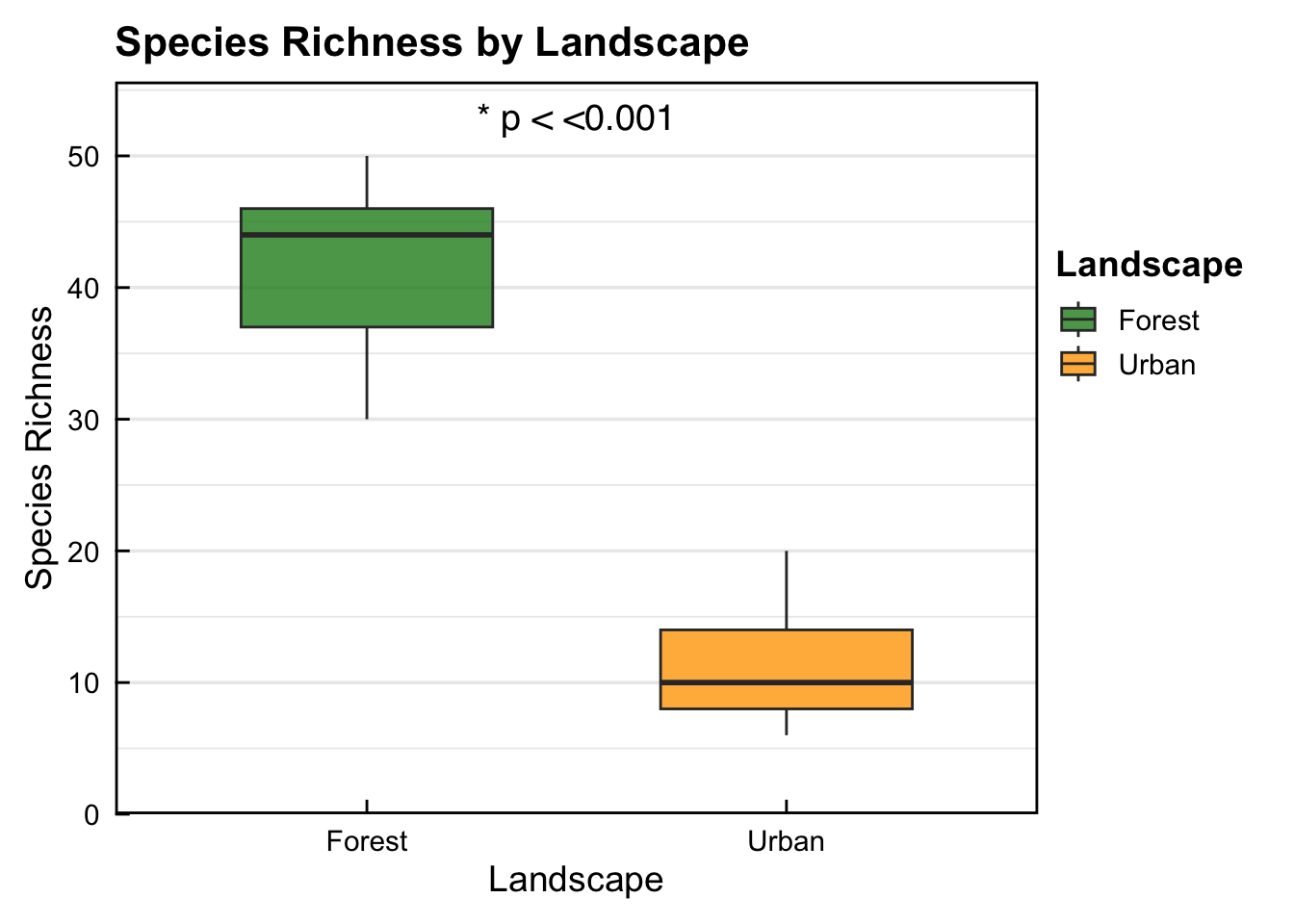

Box-plot showing that the Forest landscape (41.11) has significantly higher bird species richness compared to the Urban landscape (11.44) (p < 0.0001).

3.5 Species richness statistical comparisons by site

Calculate descriptive statistics for each site within each landscape.

# Descriptive statistics for species richness by site
site_summary_richness <- richness_df %>%
  group_by(Landscape, Site) %>%
  summarise(
    Mean = mean(Species_Richness),
    SD = sd(Species_Richness),
    SE = SD / sqrt(n())
  )
print(site_summary_richness)

# A tibble: 6 × 5
# Groups:   Landscape [2]
  Landscape Site          Mean    SD    SE
  <chr>     <chr>        <dbl> <dbl> <dbl>
1 Forest    Forest_Site1 42.3   4.73 2.73 
2 Forest    Forest_Site2 41.7   6.81 3.93 
3 Forest    Forest_Site3 39.3  10.1  5.81 
4 Urban     Urban_Site1  10.7   4.16 2.40 
5 Urban     Urban_Site2  15     6.24 3.61 
6 Urban     Urban_Site3   8.67  1.53 0.882

The descriptive summary of mean species richness for sites shows that all 3 forest sites are higher than the 3 Urban sites. But we still need to run a statistical test to check for significance

Conduct an ANOVA with Tukey’s post-hoc test to identify any significant differences in species richness between sites and where differences occur.

# ANOVA to test for significant differences in sites within  landscapes
anova_nested <- aov(Species_Richness ~ Landscape + Site %in% Landscape, data = richness_df) # TODO These is no sig dif within sites, so should probs not run the ANOVA/Tukey below - but it does provide us with the letters for the plot
summary(anova_nested)

               Df Sum Sq Mean Sq F value   Pr(>F)    
Landscape       1   3960    3960  103.92 2.91e-07 ***
Landscape:Site  4     78      19    0.51     0.73    
Residuals      12    457      38                     
---
Signif. codes:  0 '***' 0.001 '**' 0.01 '*' 0.05 '.' 0.1 ' ' 1

# ANOVA to test for significant differences between all sites across both landscapes (# TODO Check this is valid)
anova_all_sites <- aov(Species_Richness ~ Site, data = richness_df)

#Tukey's post-hoc to show where significant differences are between sites
tukey_all_sites <- TukeyHSD(anova_all_sites)
tukey_all_sites$Site

                                 diff       lwr        upr        p adj
Forest_Site2-Forest_Site1  -0.6666667 -17.59756  16.264230 0.9999925867
Forest_Site3-Forest_Site1  -3.0000000 -19.93090  13.930896 0.9894045692
Urban_Site1-Forest_Site1  -31.6666667 -48.59756 -14.735770 0.0004486064
Urban_Site2-Forest_Site1  -27.3333333 -44.26423 -10.402437 0.0016515087
Urban_Site3-Forest_Site1  -33.6666667 -50.59756 -16.735770 0.0002533679
Forest_Site3-Forest_Site2  -2.3333333 -19.26423  14.597563 0.9966532647
Urban_Site1-Forest_Site2  -31.0000000 -47.93090 -14.069104 0.0005450276
Urban_Site2-Forest_Site2  -26.6666667 -43.59756  -9.735770 0.0020339095
Urban_Site3-Forest_Site2  -33.0000000 -49.93090 -16.069104 0.0003058685
Urban_Site1-Forest_Site3  -28.6666667 -45.59756 -11.735770 0.0010955258
Urban_Site2-Forest_Site3  -24.3333333 -41.26423  -7.402437 0.0042799488
Urban_Site3-Forest_Site3  -30.6666667 -47.59756 -13.735770 0.0006012322
Urban_Site2-Urban_Site1     4.3333333 -12.59756  21.264230 0.9492760475
Urban_Site3-Urban_Site1    -2.0000000 -18.93090  14.930896 0.9983833589
Urban_Site3-Urban_Site2    -6.3333333 -23.26423  10.597563 0.8018091487

ANOVA results show a significant difference in landscape Shannon diversity but not sites within landscape. Further, output form the Tukey post-hoc test shows that there is significantly higher bird species richness in all Forest sites compared to all Urban sites. However, there is no significant difference in bird species richness between sites within the same landscape. Check table for exact significance levels for pairwise comparisons.

3.6 Plot species richness by site

letters_df <- multcompView::multcompLetters4(anova_all_sites, tukey_all_sites)
site_letters <- data.frame(Site = names(letters_df$Site$Letters),
                           Letters = letters_df$Site$Letters)
richness_df <- left_join(richness_df, site_letters, by = "Site")
y_max_rich <- max(richness_df$Species_Richness)
y_breaks_rich <- pretty(c(0, y_max_rich))
y_breaks_rich <- y_breaks_rich[y_breaks_rich >= 0]
ggplot(richness_df, aes(x = Site, y = Species_Richness, fill = Landscape)) +
  geom_boxplot(
    alpha = 0.8,
    width = 0.6,
    outlier.shape = 21,
    outlier.size = 2.5,
    outlier.stroke = 0.4,
    outlier.colour = "black"
  ) +
  geom_text(
    data = site_letters,
    aes(x = Site, y = max(richness_df$Species_Richness) + 3, label = Letters),
    inherit.aes = FALSE,
    size = 5,
    family = "sans"  
  ) +
  scale_fill_manual(values = c("Forest" = "#228B22", "Urban" = "#FFA500")) +
  scale_y_continuous(
    breaks = y_breaks_rich,
    labels = function(b) { as.character(b) },
    expand = expansion(mult = c(0, 0.05)),
    limits = c(0, NA)
  ) +
  labs(
    title = "Species Richness by Site (Grouped by Landscape)",
    x = "Site",
    y = "Species Richness",
    fill = "Landscape"
  ) +
  theme_minimal(base_size = 14) +
  theme(
    axis.text.x = element_text(color = "black", angle = 45, hjust = 1, vjust = 1, margin = margin(t = 6)),
    axis.text.y = element_text(color = "black", margin = margin(r = 6)),
    axis.ticks.length = unit(-0.2, "cm"),
    axis.ticks = element_line(color = "black", linewidth = 0.5),
    panel.grid.major.x = element_blank(),
    
    legend.position = c(1, 0.8),
    legend.justification = c("left", "top"),
    legend.box.just = "left",
    legend.background = element_blank(),
    legend.title = element_text(face = "bold"),
    
    plot.title = element_text(face = "bold", size = 16),
    plot.subtitle = element_text(size = 13),
    panel.border = element_rect(color = "black", fill = NA, linewidth = 1),
    plot.margin = margin(10, 100, 10, 10)
  ) +
  guides(fill = guide_legend(title.position = "top"))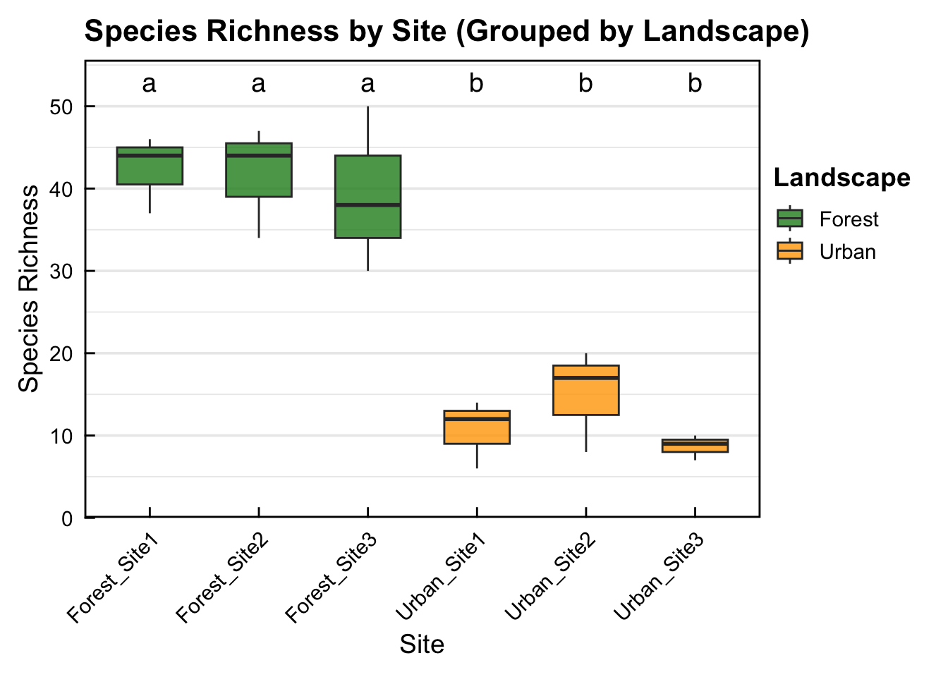

Box-plot showing that there is significantly higher bird species richness in all Forest sites compared to all Urban sites. However, there is no significant difference in bird species richness between sites within the same landscape. Sites with the same letter (e.g. a + a) indicates no significant difference in species richness, sites with different letters (e.g. a + b) display significantly different bird species richness.

3.7 Landscape temporal trend comparison

Here we investigate (via linear mixed-effect model) and visualise potential differences in species richness over a temporal scale (each sampling event throughout the year)

#Converts time into a categorical variable
richness_df$Time <- factor(richness_df$Time, levels = c("January", "May", "September"))

#Fits a linear mixed-effects model using the lmer() function (from the lmerTest package)
richness_lme <- lmer(Species_Richness ~ Time * Landscape + (1 | Site), data = richness_df)

boundary (singular) fit: see help('isSingular')

summary(richness_lme)

Linear mixed model fit by REML. t-tests use Satterthwaite's method [
lmerModLmerTest]
Formula: Species_Richness ~ Time * Landscape + (1 | Site)
   Data: richness_df

REML criterion at convergence: 79.1

Scaled residuals: 
    Min      1Q  Median      3Q     Max 
-1.2067 -0.5363 -0.2346  0.5698  1.6090 

Random effects:
 Groups   Name        Variance Std.Dev.
 Site     (Intercept)  0.00    0.000   
 Residual             24.72    4.972   
Number of obs: 18, groups:  Site, 6

Fixed effects:
                             Estimate Std. Error      df t value Pr(>|t|)    
(Intercept)                    36.000      2.871  12.000  12.541 2.96e-08 ***
TimeMay                        10.667      4.060  12.000   2.627   0.0221 *  
TimeSeptember                   4.667      4.060  12.000   1.149   0.2727    
LandscapeUrban                -23.333      4.060  12.000  -5.747 9.20e-05 ***
TimeMay:LandscapeUrban         -9.333      5.741  12.000  -1.626   0.1300    
TimeSeptember:LandscapeUrban   -9.667      5.741  12.000  -1.684   0.1181    
---
Signif. codes:  0 '***' 0.001 '**' 0.01 '*' 0.05 '.' 0.1 ' ' 1

Correlation of Fixed Effects:
            (Intr) TimeMy TmSptm LndscU TmM:LU
TimeMay     -0.707                            
TimeSeptmbr -0.707  0.500                     
LandscpUrbn -0.707  0.500  0.500              
TmMy:LndscU  0.500 -0.707 -0.354 -0.707       
TmSptmbr:LU  0.500 -0.354 -0.707 -0.707  0.500
optimizer (nloptwrap) convergence code: 0 (OK)
boundary (singular) fit: see help('isSingular')

#Post-hoc pairwise comparisons of Time within each Landscape
emmeans(richness_lme, pairwise ~ Time | Landscape)

$emmeans
Landscape = Forest:
 Time      emmean   SE df lower.CL upper.CL
 January    36.00 2.87 12    29.75     42.3
 May        46.67 2.87 12    40.41     52.9
 September  40.67 2.87 12    34.41     46.9

Landscape = Urban:
 Time      emmean   SE df lower.CL upper.CL
 January    12.67 2.87 12     6.41     18.9
 May        14.00 2.87 12     7.75     20.3
 September   7.67 2.87 12     1.41     13.9

Degrees-of-freedom method: kenward-roger 
Confidence level used: 0.95 

$contrasts
Landscape = Forest:
 contrast            estimate   SE df t.ratio p.value
 January - May         -10.67 4.06  8  -2.627  0.0701
 January - September    -4.67 4.06  8  -1.149  0.5130
 May - September         6.00 4.06  8   1.478  0.3504

Landscape = Urban:
 contrast            estimate   SE df t.ratio p.value
 January - May          -1.33 4.06  8  -0.328  0.9427
 January - September     5.00 4.06  8   1.232  0.4690
 May - September         6.33 4.06  8   1.560  0.3159

Degrees-of-freedom method: kenward-roger 
P value adjustment: tukey method for comparing a family of 3 estimates

Output from the linear mixed-effect model initially showed a significant difference in the mean species richness observed in the Forest landscape between Jan - May. However, no post-hoc pairwise comparisons were statistically significant after Tukey post-hoc correction.

3.8 Plot temporal trends of landscape species richness. This displays the mean bird species rich of sites within each landscape for each sampling event.

# Aggregate mean species richness by Landscape and Time
richness_mean <- richness_df %>%
  group_by(Landscape, Time) %>%
  summarise(Mean_Richness = mean(Species_Richness), .groups = "drop")

# Arrange Time properly
richness_mean$Time <- factor(richness_mean$Time, levels = c("January", "May", "September"))

# Create a segment dataset for mean lines
richness_segments_mean <- richness_mean %>%
  arrange(Landscape, Time) %>%
  group_by(Landscape) %>%
  mutate(
    next_richness = lead(Mean_Richness),
    next_time = lead(Time)
  ) %>%
  filter(!is.na(next_richness)) %>%
  ungroup()

richness_segments_mean <- richness_segments_mean %>%
  mutate(
    LineColor = Landscape 
  )

y_max_time <- max(richness_df$Species_Richness)
y_breaks_time <- pretty(c(0, y_max_time))

ggplot() +
  geom_segment(
    data = richness_segments_mean,
    aes(x = Time, xend = next_time, y = Mean_Richness, yend = next_richness, color = LineColor, group = Landscape),
    size = 1.5,
    show.legend = FALSE  # ❌ No legend for lines
  ) +
  geom_point(
    data = richness_mean,
    aes(x = Time, y = Mean_Richness, fill = Landscape),
    shape = 21,
    size = 5,
    stroke = 0.8,
    color = "black"  
  ) +
  scale_fill_manual(
    name = "Landscape",
    values = c(
      "Forest" = "#228B22",  
      "Urban" = "#FFA500"   
    )
  ) +
  scale_color_manual(
    values = c(
      "Forest" = "#228B22",
      "Urban" = "#FFA500"
    )
  ) +
  scale_y_continuous(
    breaks = y_breaks_time,
    labels = function(b) { as.character(b) },
    expand = expansion(mult = c(0, 0.05)),
    limits = c(0, NA)
  ) +
  labs(
    title = "Temporal Trends in Mean Species Richness by Landscape",
    x = "Time",
    y = "Mean Species Richness",
    fill = "Landscape"  
  ) +
  theme_minimal(base_size = 14) +
  theme(
    axis.ticks.length = unit(-0.2, "cm"),
    axis.ticks = element_line(color = "black", linewidth = 0.5),
    axis.text.x = element_text(color = "black", margin = margin(t = 6)),
    axis.text.y = element_text(color = "black", margin = margin(r = 6)),
    panel.grid.major.x = element_blank(),
    legend.position = c(1, 0.8),
    legend.justification = c("left", "top"),
    legend.box.just = "left",
    legend.background = element_blank(),
    legend.title = element_text(face = "bold"),
    plot.title = element_text(face = "bold", size = 14),
    panel.border = element_rect(color = "black", fill = NA, linewidth = 1),
    plot.margin = margin(10, 100, 10, 10)
  ) +
  guides(fill = guide_legend(
    title.position = "top",
    override.aes = list(shape = 21, fill = c("#228B22", "#FFA500"), color = "black", size = 5, stroke = 0.8)
  ))

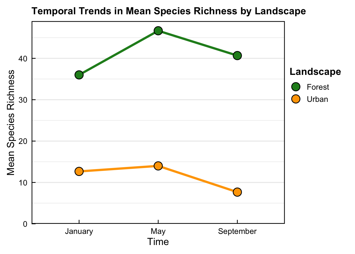
Plot trend suggests an effect of time on mean bird species richness between Jan - May in the Forest landscape, however, Tukey post-hoc analysis/correction indicated that this was not the case.

Step 4: Shannon diversity

This section will deal with Shannon diversity calculations, comparisons and visualisations.

Shannon diversity is a valuable complement to species richness because it accounts for both the number of species and their relative abundances. While richness measures how many species are present, Shannon diversity also captures how evenly individuals are distributed among those species, providing a more nuanced view of community structure.

4.1 Shannon diversity index calculations

Calculate Shannon diversity index for each sampling event in each site and landscape

# Calculate Shannon diversity for each site at each sampling event
shannon_df <- abundance_wide %>%
  mutate(Shannon = diversity(select(., starts_with("Bird")), index = "shannon")) %>%
  select(Site, Time, Landscape, SiteTime, Shannon)
# View Shannon values
head(shannon_df)

# A tibble: 6 × 5
  Site         Time      Landscape SiteTime               Shannon
  <chr>        <chr>     <chr>     <chr>                    <dbl>
1 Forest_Site1 January   Forest    Forest_Site1_January      3.73
2 Forest_Site1 May       Forest    Forest_Site1_May          3.76
3 Forest_Site1 September Forest    Forest_Site1_September    3.54
4 Forest_Site2 January   Forest    Forest_Site2_January      3.47
5 Forest_Site2 May       Forest    Forest_Site2_May          3.73
6 Forest_Site2 September Forest    Forest_Site2_September    3.79

#str(shannon_df)

Check each row of Shannon diversity calculations has been completed corrected.

4.2 Shannon diversity statistical comparisons by landscape

Descriptive statistics summary for Forest and Urban landscape bird Shannon diversity

shannon_landscape_summary <- shannon_df %>%
  group_by(Landscape) %>%
  summarise(
    Mean = mean(Shannon),
    SD = sd(Shannon),
    SE = SD / sqrt(n())
  )
print(shannon_landscape_summary)

# A tibble: 2 × 4
  Landscape  Mean    SD     SE
  <chr>     <dbl> <dbl>  <dbl>
1 Forest     3.64 0.172 0.0573
2 Urban      2.18 0.393 0.131

The descriptive summary shows that the Forest landscape (3.64) has a higher mean Shannon diversity of birds compared to the Urban landscape (2.18).

Run a t-test (Welch) to check for significant differences in Shannon diversity between landscapes

# T-test: Forest vs Urban
shannon_ttest_landscape <- t.test(Shannon ~ Landscape, data = shannon_df)
print(shannon_ttest_landscape)


    Welch Two Sample t-test

data:  Shannon by Landscape
t = 10.223, df = 10.959, p-value = 6.115e-07
alternative hypothesis: true difference in means between group Forest and group Urban is not equal to 0
95 percent confidence interval:
 1.146730 1.776317
sample estimates:
mean in group Forest  mean in group Urban 
            3.641878             2.180354

The result of the t-test shows that the Forest landscape (3.64) has significantly higher bird Shannon diversity compared to the Urban landscape (2.18) (p < 0.0001).

4.3 Plot Shannon diversity by landscape

y_max <- max(shannon_df$Shannon)
y_breaks <- pretty(c(0, y_max))
ggplot(shannon_df, aes(x = Landscape, y = Shannon, fill = Landscape)) +
  geom_boxplot(
    alpha = 0.8,
    width = 0.6,
    outlier.shape = 21,
    outlier.size = 2.5,
    outlier.stroke = 0.4,
    outlier.colour = "black"
  ) +
  scale_fill_manual(values = c("Forest" = "#228B22", "Urban" = "#FFA500")) +
  scale_y_continuous(
    breaks = y_breaks,
    labels = function(b) { as.character(b) },
    expand = expansion(mult = c(0, 0.05)),
    limits = c(0, NA)
  ) +
  annotate(
    "text",
    x = 1.5,
    y = max(shannon_df$Shannon) + 0.1,
    label = "* p < 0.001",
    size = 5,
    family = "sans"  # No bold
  ) +
  labs(
    title = "Shannon Diversity by Landscape",
    x = "Landscape",
    y = "Shannon Diversity Index",
    fill = "Landscape"
  ) +
  theme_minimal(base_size = 14) +
  theme(
    axis.ticks.length = unit(-0.2, "cm"),
    axis.ticks = element_line(color = "black", linewidth = 0.5),
    axis.text.x = element_text(margin = margin(t = 6)),
    axis.text.y = element_text(margin = margin(r = 6)),
    panel.grid.major.x = element_blank(),
    legend.position = c(1, 0.8),
    legend.justification = c("left", "top"),
    legend.box.just = "left",
    legend.background = element_blank(),
    legend.title = element_text(face = "bold"),
    plot.title = element_text(face = "bold", size = 16),
    plot.subtitle = element_text(size = 13),
    panel.border = element_rect(color = "black", fill = NA, linewidth = 1),
    plot.margin = margin(10, 100, 10, 10)
  ) +
  guides(fill = guide_legend(title.position = "top"))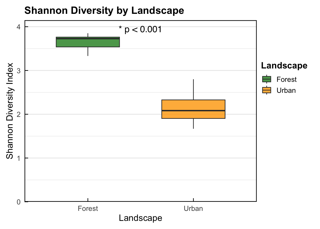

Box plot showing that the Forest landscape (3.64) has significantly higher bird Shannon diversity compared to the Urban landscape (2.18) (p < 0.0001).

4.4 Shannon diversity statistical comparisons (ANOVA) by site

#ANOVA: Sites within Landscapes
shannon_anova_nested <- aov(Shannon ~ Landscape + Site %in% Landscape, data = shannon_df)
summary(shannon_anova_nested)

               Df Sum Sq Mean Sq F value   Pr(>F)    
Landscape       1  9.612   9.612 112.260 1.91e-07 ***
Landscape:Site  4  0.444   0.111   1.296    0.326    
Residuals      12  1.027   0.086                     
---
Signif. codes:  0 '***' 0.001 '**' 0.01 '*' 0.05 '.' 0.1 ' ' 1

# All-site comparison with Tukey HSD
shannon_anova_all_sites <- aov(Shannon ~ Site, data = shannon_df)
shannon_tukey_all <- TukeyHSD(shannon_anova_all_sites)
print(shannon_tukey_all)

  Tukey multiple comparisons of means
    95% family-wise confidence level

Fit: aov(formula = Shannon ~ Site, data = shannon_df)

$Site
                                 diff        lwr        upr     p adj
Forest_Site2-Forest_Site1 -0.01267688 -0.8151930  0.7898392 0.9999999
Forest_Site3-Forest_Site1 -0.08969828 -0.8922144  0.7128178 0.9987584
Urban_Site1-Forest_Site1  -1.57171120 -2.3742273 -0.7691951 0.0002924
Urban_Site2-Forest_Site1  -1.19819363 -2.0007097 -0.3956775 0.0031577
Urban_Site3-Forest_Site1  -1.71704136 -2.5195574 -0.9145253 0.0001254
Forest_Site3-Forest_Site2 -0.07702140 -0.8795375  0.7254947 0.9994037
Urban_Site1-Forest_Site2  -1.55903431 -2.3615504 -0.7565182 0.0003155
Urban_Site2-Forest_Site2  -1.18551674 -1.9880328 -0.3830007 0.0034401
Urban_Site3-Forest_Site2  -1.70436448 -2.5068806 -0.9018484 0.0001348
Urban_Site1-Forest_Site3  -1.48201291 -2.2845290 -0.6794968 0.0005041
Urban_Site2-Forest_Site3  -1.10849534 -1.9110114 -0.3059793 0.0058243
Urban_Site3-Forest_Site3  -1.62734308 -2.4298592 -0.8248270 0.0002104
Urban_Site2-Urban_Site1    0.37351757 -0.4289985  1.1760337 0.6345096
Urban_Site3-Urban_Site1   -0.14533016 -0.9478463  0.6571859 0.9883212
Urban_Site3-Urban_Site2   -0.51884773 -1.3213638  0.2836684 0.3167198

ANOVA results show a significant difference in landscape Shannon diversity but not sites within landscape. Further, output from the Tukey post-hoc test shows that there is significantly higher bird Shannon diversity in all Forest sites compared to all Urban sites. However, there is no significant difference in bird Shannon diversity between sites within the same landscape. Check table for exact significance levels for pairwise comparisons.

4.5 Plot Shannon diversity by site

# Add significance letters
shannon_letters <- multcompView::multcompLetters4(shannon_anova_all_sites, shannon_tukey_all)
site_letters_shannon <- data.frame(Site = names(shannon_letters$Site$Letters),
                                   Letters = shannon_letters$Site$Letters)
shannon_df <- left_join(shannon_df, site_letters_shannon, by = "Site")


# ---- Shannon diversity by site ----#

y_max <- max(shannon_df$Shannon)
y_breaks <- pretty(c(0, y_max))
ggplot(shannon_df, aes(x = Site, y = Shannon, fill = Landscape)) +
  geom_boxplot(
    alpha = 0.8,
    width = 0.6,
    outlier.shape = 21,
    outlier.size = 2.5,
    outlier.stroke = 0.4,
    outlier.colour = "black"
  ) +
  geom_text(
    data = site_letters_shannon,
    aes(x = Site, y = max(shannon_df$Shannon) + 0.2, label = Letters),
    inherit.aes = FALSE,
    size = 5,
    family = "sans"
  ) +
  scale_fill_manual(values = c("Forest" = "#228B22", "Urban" = "#FFA500")) +
  scale_y_continuous(
    breaks = y_breaks,
    labels = function(b) {
    as.character(b)
    },
    expand = expansion(mult = c(0, 0.05)),
    limits = c(0, NA)
  ) +
  labs(
    title = "Shannon Diversity by Site within Landscape",
    x = "Site",
    y = "Shannon Diversity Index",
    fill = "Landscape"
  ) +
  theme_minimal(base_size = 14) +
  theme(
    axis.ticks.length = unit(-0.2, "cm"),
    axis.ticks = element_line(color = "black", linewidth = 0.5),
    axis.text.x = element_text(angle = 45, hjust = 1, vjust = 1, margin = margin(t = 6)),
    axis.text.y = element_text(margin = margin(r = 6)),
    panel.grid.major.x = element_blank(),
    legend.position = c(1, .8),
    legend.justification = c("left", "top"),
    legend.box.just = "left",
    legend.background = element_blank(),  
    legend.title = element_text(face = "bold"),
    plot.title = element_text(face = "bold", size = 16),
    plot.subtitle = element_text(size = 13),
    panel.border = element_rect(color = "black", fill = NA, linewidth = 1),
    plot.margin = margin(10, 100, 10, 10)
  )

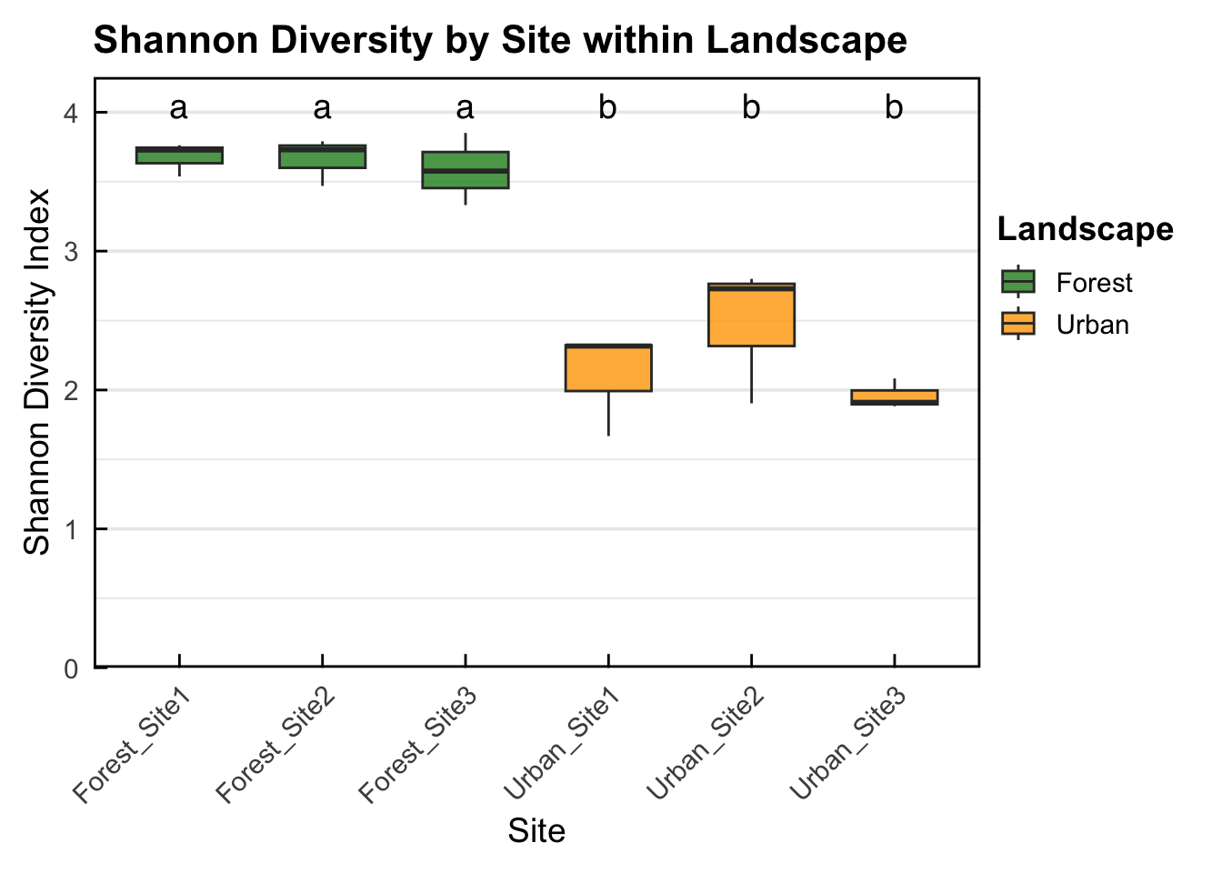
Box-plot showing that there is significantly higher bird Shannon diversity in all Forest sites compared to all Urban sites. However, there is no significant difference in bird Shannon diversity between sites within the same landscape. Sites with the same letter (e.g. a + a) indicates no significant difference in Shannon diversity, sites with different letters (e.g. a + b) display significantly different bird Shannon diversity.

Summary

In this notebook we explored how to calculate species richness and Shannon diversity. We then conducted statistical comparisons between Forest and Urban landscapes and for sites within and between these landscapes, to assess the potential impact of landscape and site on these metrics. Finally, we produced commonly used output plots to visualise the results of these comparisons.

The methodology used in this notebook could be applied to flora, fauna or other biological communities in both terrestrial or aquatic environments as an effective baseline measurement of diversity, from which extended analysis could be performed. This may include for example, species distribution models (SDMs) to further ascertain key drivers impacting the diversity and geographic distribution of the target species.

References

Chao, A., & Chiu, C.-H. (2016). Species richness: Estimation and comparison. In Wiley StatsRef: Statistics Reference Online (pp. 1–26). Wiley. https://doi.org/10.1002/9781118445112.stat03432.pub2

Fahrig, L. (2003). Effects of habitat fragmentation on biodiversity. Annual Review of Ecology, Evolution, and Systematics, 34, 487–515. https://doi.org/10.1146/annurev.ecolsys.34.011802.132419

Gotelli, N. J., & Colwell, R. K. (2001). Quantifying biodiversity: Procedures and pitfalls in the measurement and comparison of species richness. Ecology Letters, 4(4), 379–391. https://doi.org/10.1046/j.1461-0248.2001.00230.x

Gotelli, N. J., Anderson, M. J., Arita, H. T., Chao, A., Colwell, R. K., Connolly, S. R., Currie, D. J., Dunn, R. R., Graves, G. R., Green, J. L., Grytnes, J. A., Jetz, W., Lyons, S. K., McCain, C. M., Magurran, A. E., Rahbek, C., Rangel, T. F. L. V. B., Soberón, J., Webb, C. O., & Willig, M. R. (2009). Patterns and causes of species richness: a general simulation model for macroecology. Ecology Letters, 12(9), 873–886. https://doi.org/10.1111/j.1461-0248.2009.01353.x

Hill, M. O. (1973). Diversity and evenness: A unifying notation and its consequences. Ecology, 54(2), 427–432.

Magurran, A. E. (2004). Measuring biological diversity. Blackwell Science Ltd.

Shannon, C. E. (1948). A mathematical theory of communication. Bell System Technical Journal, 27(3), 379–423; 27(4), 623–656.

Turner, M. G. (1989). Landscape ecology: the effect of pattern on process. Annual Review of Ecology and Systematics, 20, 171–197. https://doi.org/10.1146/annurev.es.20.110189.001131

Turner, M. G., Gardner, R. H., & O’Neill, R. V. (2001). Landscape Ecology in Theory and Practice: Pattern and Process. Springer. https://doi.org/10.1007/978-1-4419-7402-5

EcoCommons received investment (https://doi.org/10.3565/chbq-mr75) from the Australian Research Data Commons (ARDC). The ARDC is enabled by the National Collaborative Research Infrastructure Strategy (NCRIS).

Our partner

How to Cite EcoCommons

If you use EcoCommons in your research, please cite the platform as follows:

EcoCommons Australia 2024. EcoCommons Australia – a collaborative commons for ecological and environmental modelling, Queensland Cyber Infrastructure Foundation, Brisbane, Queensland. Available at: https://data–explorer.app.ecocommons.org.au/ (Accessed: MM DD, YYYY). https://doi.org/10.3565/chbq-mr75

You can download the citation file for EcoCommons Australia here: Download the BibTeX file

Calculating and Visualising Species Richness and Shannon Diversity for Ecological Survey Data

Script and Data Information

Introduction

Key Concepts

K.1 Species richness

K.2 Shannon diversity

K.3 Landscape comparisons in ecology

Objectives

Workflow Overview

Step 1: Set-up R environment and packages

1.1 Set the working directory and create a folder for data.

1.2 Install and load required packages

Step 2: Downloading and preparing data

Step 3: Species richness

3.1 Check data structure before calculating species richness

3.2 Pivot data to wide format and to do species richness calculations

3.3 Species richness calculations

3.4 Species richness statistical comparisons by landscape

3.4 Plot species richness by landscape

3.5 Species richness statistical comparisons by site

3.6 Plot species richness by site

3.7 Landscape temporal trend comparison

3.8 Plot temporal trends of landscape species richness. This displays the mean bird species rich of sites within each landscape for each sampling event.

Step 4: Shannon diversity

4.1 Shannon diversity index calculations

4.2 Shannon diversity statistical comparisons by landscape

Run a t-test (Welch) to check for significant differences in Shannon diversity between landscapes

4.3 Plot Shannon diversity by landscape

4.4 Shannon diversity statistical comparisons (ANOVA) by site

4.5 Plot Shannon diversity by site

Summary

References

How to Cite EcoCommons

Our Partner

How to Cite EcoCommons