# Set the workspace to the current working directory
# Uncomment and replace the path below with your own working directory if needed:
# setwd("/Users/zhaoxiang/Documents/tmp/EC_GLM_notebook")

workspace <- getwd()  # Get the current working directory and store it in 'workspace'

# Increase the plot size by adjusting the options for plot dimensions in the notebook output
options(repr.plot.width = 16, repr.plot.height = 8)  # Sets width to 16 and height to 8 for larger plots
Species Distribution Analysis - Generalised Linear Model (GLM)
Author details: Abhimanyu Raj Singh and Xiang Zhao
Editor details: Dr Sebastian Lopez Marcano
Contact details: support@ecocommons.org.au
Copyright statement: This script is the product of the EcoCommons platform. Please refer to the EcoCommons website for more details: https://www.ecocommons.org.au/
Date: December 2024
Script information
This notebook, developed by the EcoCommons team, showcases how to build Species Distribution Models (SDMs) using Generalised Linear Model algorithm.
Other file formats of this notebook
| Notebook | Files | Open in Colab / ARDC Jupyter | DOI |
|---|---|---|---|
| GLM |   |
Introduction
Using Mountain Ash (Eucalyptus regnans), a very tall and straight tree species native to Victoria and Tasmania, we will guide you through a standard protocol developed by Zurell et al. (2020) for building species distribution models (SDMs) with one of the most widely used algorithms: the Generalised Linear Model (GLM).
Objectives
- Understand a standard protocol of species distribution models.
- Familiarise your with the five main steps of running Generalised Linear Models for a tree species.
- Learn how to adjust this Quarto Markdown notebook to run your own GLM-based SDM.
- Get accustomed to the style of the EcoCommons Notebooks.
Workflow Overview
Following a standard protocol for species distribution models proposed by Zurell et al., (2020), a R environment set-up step and five main modelling steps are demonstrated in this notebook:
| Step | Main Step | Sub-steps |
|---|---|---|
| Set-up | Set-up | S.1 Set up the working directory S.2 Install and load required R packages for this notebook S.3 Download the case study datasets |
| Step 1 | Overview and Conceptualisation | 1.1 Model objective 1.2 Taxon, location, predictors, scale |
| Step 2 | Data | 2.1 Biodiversity data 2.2 Pseudo absence data 2.3 Environmental data 2.4 Combine data |
| Step 3 | Model fitting | 3.1 Multicollinearity and variable selection 3.2 Data splitting 3.3 Model fitting |
| Step 4 | Evaluation | 4.1 Interpretation 4.2 Cross-valiadation |
| Step 5 | Predictions | 5.1 Mapping |
In the near future, this material may form part of comprehensive support materials available to EcoCommons users. If you have any corrections or suggestions to improve the efficiency, please contact the EcoCommons team.

Set-up: R Environment and Packages
Some housekeeping before we start. This process might take some time as many packages needed to be installed.
S.1 Set the working directory and create a folder for data.
Save the Quarto Markdown file (.QMD) to a folder of your choice, and then set the path to your folder as your working directory.
Ideally, you would use the renv package to create an isolated environment for installing all the required R packages used in this notebook. However, since installing renv and its dependencies can be time-consuming, we recommend trying this after the workshop.
# # Ensure "renv" package is installed
# if (!requireNamespace("renv", quietly = TRUE)) {
#   install.packages("renv")
# }
#
# # Check if renv has been initialized in the project
# if (!file.exists("renv/activate.R")) {
#   message("renv has not been initiated in this project. Initializing now...")
#   renv::init()  # Initialize renv if not already set up
# } else {
#   source("renv/activate.R")  # Activate the renv environment
#   message("renv is activated.")
# }
#
# # Check for the existence of renv.lock and restore the environment
# if (file.exists("renv.lock")) {
#   message("Restoring renv environment from renv.lock...")
#   renv::restore()
# } else {
#   message("No renv.lock file found in the current directory. Skipping restore.")
# }
S.2 Install and load essential libraries.
Install and load R packages.
# Set CRAN mirror
options(repos = c(CRAN = "https://cran.rstudio.com/"))

# List of packages to check, install if needed, and load
packages <- c("dplyr", "terra", "sf", "googledrive", "ggplot2", "corrplot", "pROC", "dismo", "spatstat.geom", "patchwork", "biomod2", "leaflet", "car", "gridExtra", "htmltools", "RColorBrewer")

# Function to display a cat message
cat_message <- function(pkg, message_type) {
  if (message_type == "installed") {
    cat(paste0(pkg, " has been installed successfully!\n"))
  } else if (message_type == "loading") {
    cat(paste0(pkg, " is already installed and has been loaded!\n"))
  }
}

# Install missing packages and load them
for (pkg in packages) {
  if (!requireNamespace(pkg, quietly = TRUE)) {
    install.packages(pkg)
    cat_message(pkg, "installed")
  } else {
    cat_message(pkg, "loading")
  }
  library(pkg, character.only = TRUE)
}
dplyr is already installed and has been loaded!terra is already installed and has been loaded!sf is already installed and has been loaded!googledrive is already installed and has been loaded!
ggplot2 is already installed and has been loaded!corrplot is already installed and has been loaded!pROC is already installed and has been loaded!dismo is already installed and has been loaded!spatstat.geom is already installed and has been loaded!patchwork is already installed and has been loaded!biomod2 is already installed and has been loaded!leaflet is already installed and has been loaded!
car is already installed and has been loaded!gridExtra is already installed and has been loaded!htmltools is already installed and has been loaded!RColorBrewer is already installed and has been loaded!# If you are using renv, you can snapshot the renv after loading all the packages.
#renv::snapshot()S.3 Download case study datasets
We have prepared the following data and uploaded them to our Google Drive for your use:
Species occurrence data: Shapefile format (.shp)
Environmental variables: Stacked Raster format (.tif)
Study area boundary: Shapefile format (.shp)
# De-authenticate Google Drive to access public files
drive_deauth()

# Define Google Drive file ID and the path for downloading
zip_file_id <- "1twKlNokB7t33QH2KesH7BHYffp5kvoiP" # Replace with the actual file ID of the zipped file
datafolder_path <- file.path(workspace)

# Create a local path for the zipped file
zip_file_path <- file.path(datafolder_path, "mountain_ash_centralhighlands_data.zip")

# Function to download a file with progress messages
download_zip_file <- function(file_id, file_path) {
  cat("Downloading zipped file...\n")
  drive_download(as_id(file_id), path = file_path, overwrite = TRUE)
  cat("Downloaded zipped file to:", file_path, "\n")
}

# Create local directory if it doesn't exist
if (!dir.exists(datafolder_path)) {
  dir.create(datafolder_path, recursive = TRUE)
}

# Download the zipped file
cat("Starting to download the zipped file...\n")
Starting to download the zipped file...download_zip_file(zip_file_id, zip_file_path)Downloading zipped file...File downloaded:• 'mountain_ash_centralhighlands-20241204T022054Z-001.zip'
<id: 1twKlNokB7t33QH2KesH7BHYffp5kvoiP>Saved locally as:• '/Users/xiangzhaoqcif/dev/notebook-blog/notebooks/EC_GLM/mountain_ash_centralhighlands_data.zip'Downloaded zipped file to: /Users/xiangzhaoqcif/dev/notebook-blog/notebooks/EC_GLM/mountain_ash_centralhighlands_data.zip # Unzip the downloaded file
cat("Unzipping the file...\n")Unzipping the file...unzip(zip_file_path, exdir = datafolder_path)
cat("Unzipped files to folder:", datafolder_path, "\n")Unzipped files to folder: /Users/xiangzhaoqcif/dev/notebook-blog/notebooks/EC_GLM 1 Overview and Conceptualisation
1.1 Taxon, location, data and scale
Taxon: Mountain Ash (Eucalyptus regnans)

Photographer: Reiner Richter, ALA
Mountain Ash (Eucalyptus regnans), is a remarkably tall and straight tree native to Victoria and Tasmania. This species thrives in cool, temperate rainforests characterized by high rainfall, deep, well-drained soils, mild temperatures, and high humidity. It is typically found at altitudes ranging from 200 to 1,000 meters above sea level (Burns et al., 2015).
The Mountain Ash faces two main forms of disturbance: bushfires, which are its primary natural disturbance, and logging, which represents the primary human-induced threat to its habitat (Burns et al., 2015; Nevill et al., 2010).
Location: the Central Highlands (study area) in the south part of Victoria
Spatial and temporal scales: small (spatial) and static (temporal)
# Load your shapefiles
central_highlands <- st_read("mountain_ash_centralhighlands/central_highlands.shp")
Reading layer `central_highlands' from data source
`/Users/xiangzhaoqcif/dev/notebook-blog/notebooks/EC_GLM/mountain_ash_centralhighlands/central_highlands.shp'
using driver `ESRI Shapefile'
Simple feature collection with 1 feature and 4 fields
Geometry type: POLYGON
Dimension: XY
Bounding box: xmin: 144.9398 ymin: -38.20964 xmax: 146.4563 ymax: -36.97746
Geodetic CRS: GDA94# Custom CSS for a smaller legend box
custom_css <- tags$style(HTML("
.leaflet-control .legend {
font-size: 8px !important; /* Reduce font size */
padding: 4px; /* Reduce padding inside the legend box */
line-height: 1; /* Reduce spacing between lines */
width: auto; /* Automatically size the legend box */
height: auto; /* Automatically size the legend box */
}
.leaflet-control .legend i {
width: 10px; /* Smaller legend icons */
height: 10px;
}
"))
# Render the map
leaflet() %>%
addProviderTiles(providers$Esri.WorldImagery) %>%
# Add the Central Highlands layer with a distinct color
addPolygons(
data = central_highlands,
color = "lightblue", # Border color of Central Highlands polygon
weight = 1, # Border width
fillColor = "lightblue", # Fill color of Central Highlands
fillOpacity = 0.3, # Transparency for fill
group = "Central Highlands"
) %>%
setView(lng = 145.7, lat = -37.5, zoom = 7) %>% # Set the view to desired location
addLegend(
position = "bottomright",
colors = c("lightblue"),
labels = c("Central Highlands"),
opacity = 0.7
) %>%
# Add the custom CSS to modify the legend font size
htmlwidgets::prependContent(custom_css)1.2 Model objective
Explanation: To conduct detailed analyses of species–environment relationships and test specific hypotheses about the main factors driving species distributions.
Mapping/interpolating: To use the estimated species-environment relationships to map the distribution of the targeted species in the same geographic area.
Prediction in new area: To forecast or project the estimated species–environment relationships to a different geographic area. (Exercise, data provided)
2. Data
In this section, details about the species and environmental data, data partitioning and transfer data are provided.
2.1 Biodiversity data
Understanding your species is essential. This includes knowing their common names (which may include multiple names) and scientific name to ensure you collect the most comprehensive records available in open-access biodiversity data portals, such as the Atlas of Living Australia (ALA) or the Global Biodiversity Information Facility (GBIF).
For this exercise, we have prepared a species occurrence data file in CSV format, which was downloaded from ALA. To make it accessible, we have stored this file in the EcoCommons Public Google Drive for you to download and use conveniently.
# Read the shapefile for mountain ash occurrence point dataset
mountain_ash_centralhighlands <- st_read("mountain_ash_centralhighlands/mountain_ash_centralhighlands.shp")
Reading layer `mountain_ash_centralhighlands' from data source
`/Users/xiangzhaoqcif/dev/notebook-blog/notebooks/EC_GLM/mountain_ash_centralhighlands/mountain_ash_centralhighlands.shp'
using driver `ESRI Shapefile'
Simple feature collection with 3933 features and 1 field
Geometry type: POINT
Dimension: XY
Bounding box: xmin: 145.0258 ymin: -38.2 xmax: 146.4333 ymax: -37.22625
Geodetic CRS: GDA94# Filter the data to include only PRESENT points
mountain_ash_present <- mountain_ash_centralhighlands %>%
dplyr::filter(occrrnS == "1")
leaflet() %>%
addProviderTiles(providers$Esri.WorldImagery) %>%
# Add the Central Highlands layer with a distinct color
addPolygons(
data = central_highlands,
color = "lightblue", # Border color of Central Highlands polygon
weight = 1, # Border width
fillColor = "lightblue", # Fill color of Central Highlands
fillOpacity = 0.3, # Transparency for fill
group = "Central Highlands"
) %>%
# Add Mountain Ash presence points
addCircleMarkers(
data = mountain_ash_present,
color = "#11aa96",
radius = 1,
weight = 0.5,
opacity = 1,
fillOpacity = 1,
group = "Mountain Ash Presence Records"
) %>%
setView(lng = 145.7, lat = -37.5, zoom = 7) %>% # Adjust longitude, latitude, and zoom as needed
# Add layer controls for easier toggling
addLayersControl(
overlayGroups = c("Central Highlands", "Mountain Ash Presence Records"),
options = layersControlOptions(collapsed = FALSE)
) %>%
# Add a compact legend with a clean style
addControl(
html = "
<div style='background-color: white; padding: 4px; font-size: 8px; border: none; box-shadow: none;'>
<div style='display: flex; align-items: center; margin-bottom: 3px;'>
<div style='background: lightblue; width: 10px; height: 10px; margin-right: 5px; opacity: 0.7;'></div>
Central Highlands
</div>
<div style='display: flex; align-items: center;'>
<div style='background: #11aa96; width: 10px; height: 10px; margin-right: 5px;'></div>
Mountain Ash Presence Records
</div>
</div>
",
position = "bottomright"
)2.2 Pseudo Absence Data
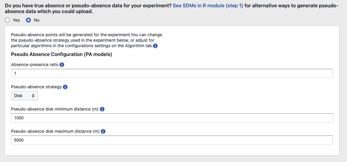
Species distribution models typically require both presence and absence data to predict the distribution of a species. However, true absence data—locations where the species is confirmed not to occur—are often unavailable for various reasons. In such cases, pseudo-absence data are used to fill this gap.
We generated pseudo-absence data using the EcoCommons platform with the following configuration:
Dispersal Kernel
Key point: Mountain Ash seed dispersal is likely within 150 meters, based on von Takach Dukai (2019).
Implication: This distance should be factored into pseudo-absence generation to avoid selecting pseudo-absence points too close to presence points, which could bias the model by including areas that the species might still occupy but haven’t been sampled.
Absence-Presence Ratio
Key point: The ratio of absence to presence is set to 1.
Implication: For each presence point, one pseudo-absence point should be generated. This balanced ratio ensures the model isn’t skewed by an overabundance of either class and aids in robust statistical comparisons.
Pseudo-Absence Strategy
Key point: Disk strategy with a range of 1000 - 5000 meters.
Implication:
The disk strategy selects pseudo-absences outside a certain buffer zone from presence points.
The range of 1000–5000 meters should be carefully reviewed since it must balance avoiding areas within the species’ potential dispersal kernel (150 meters) and including areas beyond the likely range of colonization.
# Filter the data to include only ABSENT points
mountain_ash_absent <- mountain_ash_centralhighlands %>%
  dplyr::filter(occrrnS == "0")

leaflet() %>%
  addProviderTiles(providers$Esri.WorldImagery) %>%
 # Add the Central Highlands layer with a distinct color
  addPolygons(data = central_highlands,
              color = "lightblue",         # Border color of Central Highlands polygon
              weight = 1,            # Border width
              fillColor = "lightblue",  # Fill color of Central Highlands
              fillOpacity = 0.3,     # Transparency for fill
              group = "Central Highlands") %>%

    # Add Mountain Ash presence points
  addCircleMarkers(data = mountain_ash_present,
                   color = "#11aa96",
                   radius = 1,
                   weight = 0.5,
                   opacity = 1,
                   fillOpacity = 1,
                   group = "Mountain Ash Presence Records") %>%


      # Add Mountain Ash absent points
  addCircleMarkers(data = mountain_ash_absent,
                   color = "#f6aa70",
                   radius = 1,
                   weight = 0.5,
                   opacity = 1,
                   fillOpacity = 1,
                   group = "Mountain Ash Pseudo_absent Records") %>%

  setView(lng = 145.7, lat = -37.5, zoom = 7)  %>% # Adjust longitude, latitude, and zoom as needed

    # Add layer controls for easier toggling
  addLayersControl(
    overlayGroups = c("Central Highlands", "Mountain Ash Presence Records", "Mountain Ash Pseudo_absent Records"),
    options = layersControlOptions(collapsed = FALSE)
  ) %>%

  # Add a legend for the layers
  addControl(
    html = "
    <div style='background-color: white; padding: 10px; border-radius: 5px;'>
      <strong>Legend</strong><br>
      <i style='background: lightblue; width: 18px; height: 18px; display: inline-block; margin-right: 8px; opacity: 0.7;'></i>
      Central Highlands<br>
      <i style='background: #11aa96; width: 10px; height: 10px; border-radius: 50%; display: inline-block; margin-right: 8px;'></i>
      Mountain Ash Presence Records<br>
      <i style='background: #f6aa70; width: 10px; height: 10px; border-radius: 50%; display: inline-block; margin-right: 8px;'></i>
      Mountain Ash Pseudo-absent Records
    </div>
    ",
    position = "bottomright"
  )
2.3 Environmental Data
When selecting environmental variables for a model, it is important to avoid indiscriminately including any available data. Instead, select variables thoughtfully, guided by ecological knowledge and the specific hypotheses being tested.
As previously mentioned, Mountain Ash thrives in cool, temperate rainforests characterized by high rainfall, deep, well-drained soils, mild temperatures, and high humidity. This species is typically found at altitudes ranging from 200 to 1,000 meters above sea level (Burns et al., 2015). Mountain Ash habitats face two primary forms of disturbance: bushfires, which are the main natural disturbance, and logging, which constitutes the primary human-induced threat (Burns et al., 2015; Nevill et al., 2010).
| Environmental Variables Categories | Variables | Data Type | Source |
|---|---|---|---|
| Temperature and Radiation | Bioclim 01: Annual mean temperature Bioclim 04: Temperature Seasonality (standard deviation *100) Bioclim 06: Min Temperature of Coldest Month Bioclim 20: Annual mean radiation |
Continuous | 1976-2005, CSIRO via EcoCommons |
| Humidity | Bioclim 12: Annual Precipitation Bioclim 18: Precipitation of Warmest Quarter Bioclim 19: Precipitation of Coldest Quarter Bioclim 28: Annual mean moisture index Bioclim 34: Mean moisture index of warmest quarter Bioclim 35: Mean moisture index of coldest quarter |
Continuous | 1976-2005, CSIRO via EcoCommons |
| Topography | Digital Elevation Model | Continuous | Geoscience Australia via EcoCommons |
| Soil | Australian Soil Classification | Categorical | Tern via EcoCommons |
| Disturbance | Fires Logging |
Continuous | Vic DEECA spatial data and resources |
# Load the stacked raster layers
env_var_stack <- rast("mountain_ash_centralhighlands/central_highlands_15envvar.tif")

# Define the custom names for the raster layers
layer_names <- c(
  "Annual_Mean_Temp",
  "Temp_Seasonality",
  "Min_Temp_Coldest_Month",
  "Mean_Temp_Warmest_Quarter",
  "Annual_Mean_Radiation",
  "Annual_Precipitation",
  "Precip_Warmest_Quarter",
  "Precip_Coldest_Quarter",
  "Annual_Mean_Moisture",
  "Moisture_Warmest_Quarter",
  "Moisture_Coldest_Quarter",
  "Elevation",
  "Soil_Type",
  "Fires",
  "Logging"
)


# Assign the custom names to the raster layers
names(env_var_stack) <- layer_names

# We want to make sure that soil type raster layer is factor.
env_var_stack[["Soil_Type"]] <- as.factor(env_var_stack[["Soil_Type"]])

# Check if the names are assigned correctly
print(names(env_var_stack))
[1] "Annual_Mean_Temp" "Temp_Seasonality"
[3] "Min_Temp_Coldest_Month" "Mean_Temp_Warmest_Quarter"
[5] "Annual_Mean_Radiation" "Annual_Precipitation"
[7] "Precip_Warmest_Quarter" "Precip_Coldest_Quarter"
[9] "Annual_Mean_Moisture" "Moisture_Warmest_Quarter"
[11] "Moisture_Coldest_Quarter" "Elevation"
[13] "Soil_Type" "Fires"
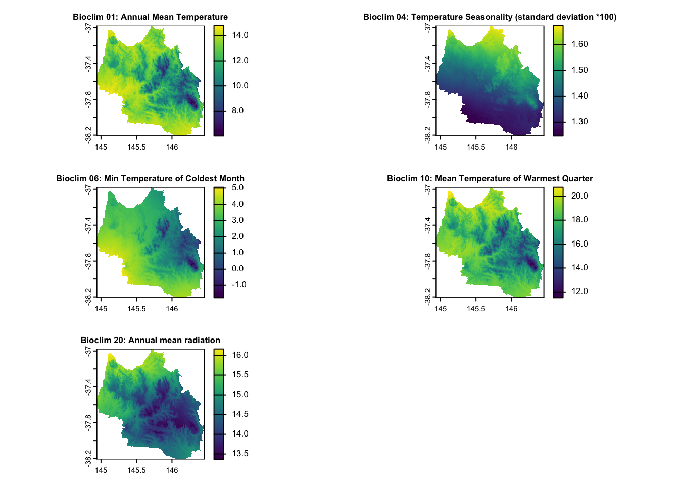
[15] "Logging" # Custom titles for the layers
layer_titles <- c(
"Bioclim 01: Annual Mean Temperature",
"Bioclim 04: Temperature Seasonality (standard deviation *100)",
"Bioclim 06: Min Temperature of Coldest Month",
"Bioclim 10: Mean Temperature of Warmest Quarter",
"Bioclim 20: Annual mean radiation"
)
# Indices of the layers to plot
layers_to_plot <- c(1, 2, 3, 4, 8)
# Set layout for plotting (3 rows, 2 columns for 5 plots)
par(mfrow = c(3, 2))
# Plot each specified layer with its custom title and smaller title size
for (i in seq_along(layers_to_plot)) {
layer_index <- layers_to_plot[i]
plot(env_var_stack[[layer_index]], main = layer_titles[i], cex.main = 0.8) # Adjust cex.main for title size
}
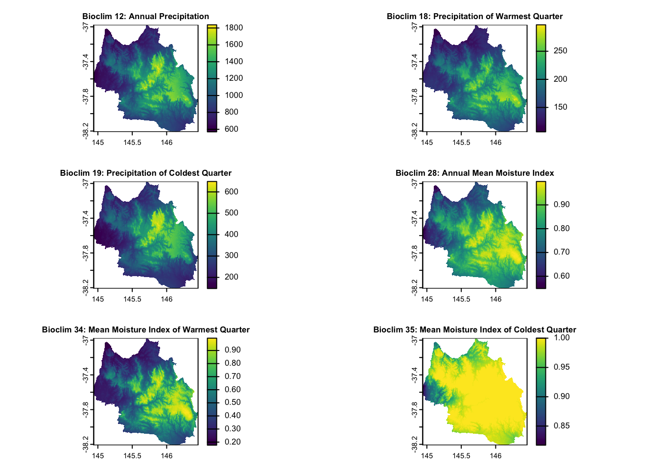
# Custom titles for the specified layers
layer_titles <- c(
  "Bioclim 12: Annual Precipitation",
  "Bioclim 18: Precipitation of Warmest Quarter",
  "Bioclim 19: Precipitation of Coldest Quarter",
  "Bioclim 28: Annual Mean Moisture Index",
  "Bioclim 34: Mean Moisture Index of Warmest Quarter",
  "Bioclim 35: Mean Moisture Index of Coldest Quarter"
)

# Indices of the layers to plot
layers_to_plot <- c(5, 6, 7, 9, 10, 11)

# Set layout for plotting (3 rows, 2 columns for 5 plots)
par(mfrow = c(3, 2))

# Plot each specified layer with its custom title and smaller title size
for (i in seq_along(layers_to_plot)) {
  layer_index <- layers_to_plot[i]
  plot(env_var_stack[[layer_index]], main = layer_titles[i], cex.main = 0.8) # Adjust cex.main for title size
}
# Custom titles for the specified layers
layer_titles <- c(
  "Digital Elevation Model",
  "Australian Soil Classification",
  "Logging",
  "Fires"
)

# Indices of the layers to plot
layers_to_plot <- c(12:15)

# Set layout for plotting (3 rows, 2 columns for 5 plots)
par(mfrow = c(2, 2))

# Plot each specified layer with its custom title and smaller title size
for (i in seq_along(layers_to_plot)) {
  layer_index <- layers_to_plot[i]
  plot(env_var_stack[[layer_index]], main = layer_titles[i], cex.main = 0.8) # Adjust cex.main for title size
}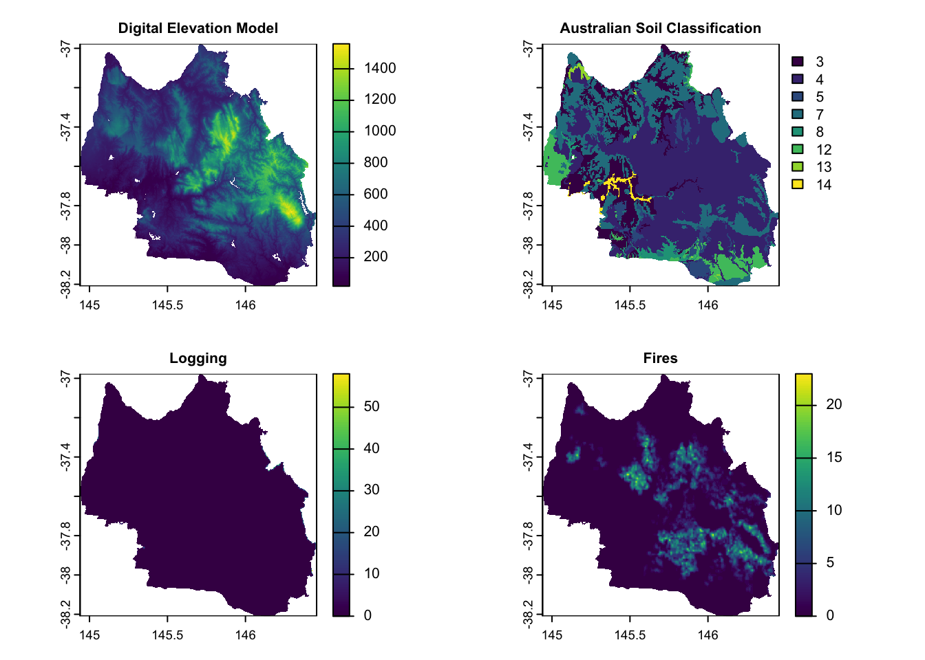
Soil Type Classification: 3 - Dermosol, 4 - Chromosol, 5 - Ferrosol, 7 - Tenosol, 8 - Kandosol,12 - Calcarosol, 13 - Organosol, and 14 - Anthroposol.
2.4 Combine species occurrence data and environmental variables
We will create a data frame that combines each presence/absence record of Mountain Ash with data from our 15 environmental variables.
# Convert species occurrence data to terra-compatible SpatVector
occurrence_vect <- vect(mountain_ash_centralhighlands)

# Extract raster values at species occurrence points
extracted_values <- terra::extract(env_var_stack, occurrence_vect)

# Combine occurrence data with extracted raster values
# (Keep geometry or drop it based on your needs)
occurrence_data <- cbind(as.data.frame(mountain_ash_centralhighlands), extracted_values)

# Remove rows with any NA values in predictors
occurrence_data <- na.omit(occurrence_data)

# we want to make sure the data type of soil types is factor.
occurrence_data$Soil_Type <- as.factor(occurrence_data$Soil_Type)

head(occurrence_data)
occrrnS geometry ID Annual_Mean_Temp Temp_Seasonality
1 1 POINT (145.7339 -37.67417) 1 10.369396 1.424792
2 1 POINT (146.1373 -37.7804) 2 8.822482 1.449565
3 1 POINT (145.3817 -37.88166) 3 12.967784 1.280466
4 1 POINT (146.1797 -37.84517) 4 10.826058 1.390526
5 1 POINT (145.3362 -37.88002) 5 11.825127 1.278574
6 1 POINT (145.9281 -37.83222) 6 10.293063 1.386414
Min_Temp_Coldest_Month Mean_Temp_Warmest_Quarter Annual_Mean_Radiation
1 2.0631714 15.60523 1578.439
2 0.4309082 14.10276 1577.427
3 4.2351027 17.71625 1133.458
4 1.5544521 15.95073 1583.145
5 3.9153066 16.52677 1266.487
6 1.6763960 15.38035 1609.709
Annual_Precipitation Precip_Warmest_Quarter Precip_Coldest_Quarter
1 250.6433 530.1663 13.70784
2 268.0575 503.1617 13.63218
3 203.8828 331.7352 14.27531
4 275.0496 479.6527 13.56016
5 230.7354 364.2117 13.97706
6 267.1724 513.3069 13.54408
Annual_Mean_Moisture Moisture_Warmest_Quarter Moisture_Coldest_Quarter
1 0.9548221 0.8892441 1.0000000
2 0.9821509 0.9541187 1.0000000
3 0.8531148 0.6036963 0.9996078
4 0.9700990 0.9209611 1.0000000
5 0.9097116 0.7599657 1.0000000
6 0.9698939 0.9229909 1.0000000
Elevation Soil_Type Fires Logging
1 834.7029 4 0 0
2 1058.5144 4 0 3
3 314.3798 4 0 0
4 658.4626 7 0 9
5 544.9786 4 0 0
6 902.7314 4 0 73 Model fitting
3.1 Multicollinearity and Variable Selection
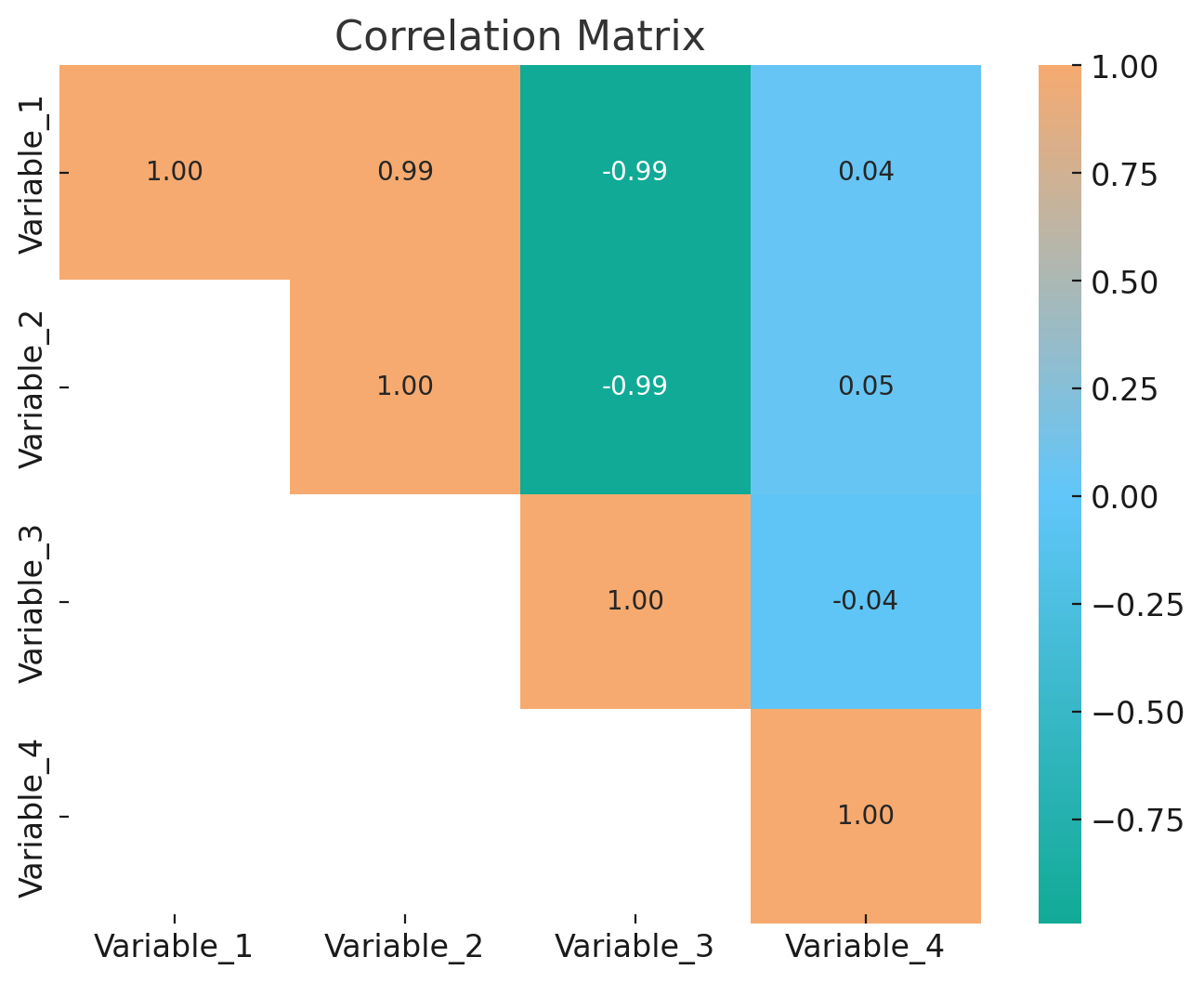
Testing for collinearity among continuous variables is an important step in many modeling processes, particularly in species distribution modeling and other regression-based analyses. Codllinearity occurs when two or more predictor variables in a dataset are highly correlated, which can lead to unstable estimates of regression coefficients and make it difficult to interpret the results.
There are two common methods for testing collinearity among continuous variables.
Correlation matrix.
layer_names <- c(
  "Annual_Mean_Temp",
  "Temp_Seasonality",
  "Min_Temp_Coldest_Month",
  "Mean_Temp_Warmest_Quarter",
  "Annual_Mean_Radiation",
  "Annual_Precipitation",
  "Precip_Warmest_Quarter",
  "Precip_Coldest_Quarter",
  "Annual_Mean_Moisture",
  "Moisture_Warmest_Quarter",
  "Moisture_Coldest_Quarter",
  "Elevation",
  "Fires",
  "Logging"
)


# Select columns by their names
cor_data <- occurrence_data[, layer_names]

# Check the structure of the numeric data
str(cor_data)
'data.frame': 3932 obs. of 14 variables:
$ Annual_Mean_Temp : num 10.37 8.82 12.97 10.83 11.83 ...
$ Temp_Seasonality : num 1.42 1.45 1.28 1.39 1.28 ...
$ Min_Temp_Coldest_Month : num 2.063 0.431 4.235 1.554 3.915 ...
$ Mean_Temp_Warmest_Quarter: num 15.6 14.1 17.7 16 16.5 ...
$ Annual_Mean_Radiation : num 1578 1577 1133 1583 1266 ...
$ Annual_Precipitation : num 251 268 204 275 231 ...
$ Precip_Warmest_Quarter : num 530 503 332 480 364 ...
$ Precip_Coldest_Quarter : num 13.7 13.6 14.3 13.6 14 ...
$ Annual_Mean_Moisture : num 0.955 0.982 0.853 0.97 0.91 ...
$ Moisture_Warmest_Quarter : num 0.889 0.954 0.604 0.921 0.76 ...
$ Moisture_Coldest_Quarter : num 1 1 1 1 1 ...
$ Elevation : num 835 1059 314 658 545 ...
$ Fires : num 0 0 0 0 0 0 5 0 0 0 ...
$ Logging : num 0 3 0 9 0 7 0 4 8 4 ...# Calculate the correlation matrix for the numeric columns
cor_matrix <- cor(cor_data, use = "complete.obs", method = "pearson")
corrplot(cor_matrix,
method = "color", # Use colored squares for correlation
type = "upper", # Show upper triangle only
order = "hclust", # Reorder variables hierarchically
addCoef.col = "black", # Show correlation coefficients in black
number.cex = 0.5, # Reduce the size of correlation labels
tl.col = "black", # Text label color
tl.srt = 30, # Rotate labels slightly for readability
tl.cex = 0.5, # Reduce text size of variable labels (set smaller valu)
cl.cex = 0.8, # Reduce text size of color legend
diag = FALSE, # Hide diagonal
col = colorRampPalette(c("#11aa96", "#61c6fa", "#f6aa70"))(200),
sig.level = 0.01, insig = "blank")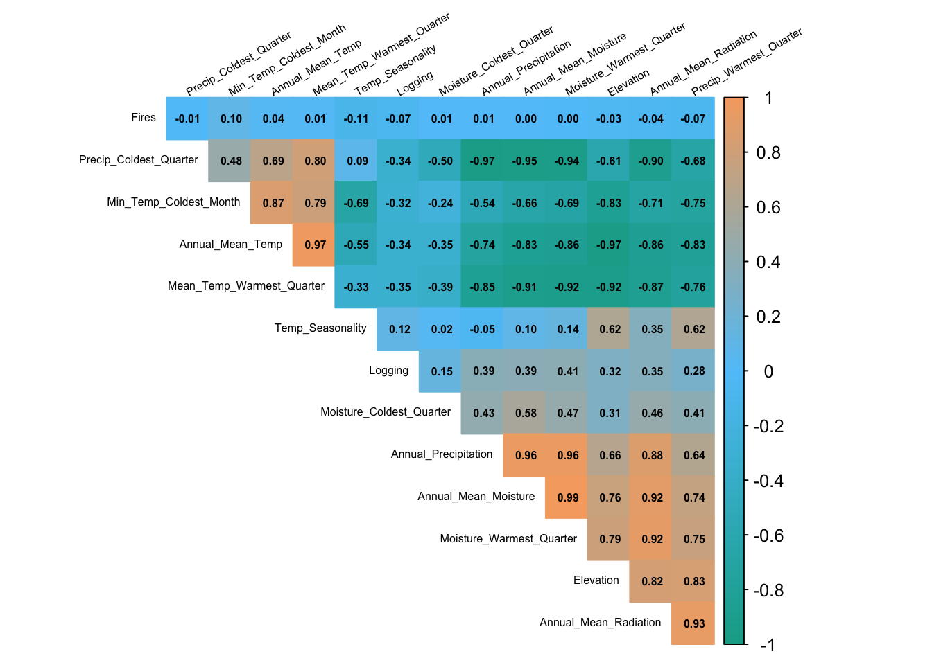
If you find corrplot is hard for you to make decisions, we can use Variance Inflation Factor (VIF). VIF is another statistical measure used to detect multicollinearity in a set of explanatory (independent) variables in a regression model.
Interpretation:
VIF = 1: No correlation
VIF > 1 and <= 5: Moderate correlation; may not require corrective action.
VIF > 5: Indicates high correlation. Multicollinearity may be problematic, and further investigation is recommended.
VIF > 10: Strong multicollinearity. The variable is highly collinear with others, and steps should be taken to address this.
# Fit a GLM for species distribution
glm_model <- glm(
  occrrnS ~ Annual_Mean_Temp + Temp_Seasonality + Min_Temp_Coldest_Month +
    Mean_Temp_Warmest_Quarter + Annual_Mean_Radiation + Annual_Precipitation +
    Precip_Warmest_Quarter + Precip_Coldest_Quarter + Annual_Mean_Moisture +
    Moisture_Warmest_Quarter + Moisture_Coldest_Quarter + Elevation + Fires + Logging,
  data = occurrence_data,
  family = binomial(link = "logit")  # Logistic regression
)
# Calculate VIF for the GLM
vif_values <- vif(glm_model)
# Convert VIF values to a data frame with two columns
vif_table <- data.frame(
Variable = names(vif_values), # Column 1: Variable names
VIF = round(vif_values, 2) # Column 2: VIF values rounded to 2 decimals
)
# Rank the VIF table from high to low
vif_table <- vif_table[order(vif_table$VIF, decreasing = TRUE), ]
# Print the ranked table
print(vif_table) Variable VIF
Annual_Mean_Temp Annual_Mean_Temp 30369.96
Mean_Temp_Warmest_Quarter Mean_Temp_Warmest_Quarter 21826.71
Annual_Mean_Radiation Annual_Mean_Radiation 2863.99
Annual_Mean_Moisture Annual_Mean_Moisture 1625.31
Temp_Seasonality Temp_Seasonality 1527.84
Moisture_Warmest_Quarter Moisture_Warmest_Quarter 1241.81
Precip_Warmest_Quarter Precip_Warmest_Quarter 1228.60
Precip_Coldest_Quarter Precip_Coldest_Quarter 562.37
Annual_Precipitation Annual_Precipitation 308.52
Elevation Elevation 42.83
Min_Temp_Coldest_Month Min_Temp_Coldest_Month 24.07
Moisture_Coldest_Quarter Moisture_Coldest_Quarter 3.80
Logging Logging 1.27
Fires Fires 1.03Rules of thumb for VIF:
Variables to Drop (Initial Recommendation):
Annual_Mean_Temp(High VIF + highly correlated with many others).Mean_Temp_Warmest_Quarter(High VIF + redundant withMin_Temp_Coldest_Month).Annual_Mean_Radiation(High VIF + redundant withElevation).Annual_Precipitation(Redundant withAnnual_Mean_Moisture).Precip_Warmest_Quarter(Redundant withMoisture_Warmest_Quarter).
Getting rid of some highly correlated variables and run VIF again.
# Fit a GLM for testing the VIF
glm_model <- glm(
occrrnS ~ Temp_Seasonality + Min_Temp_Coldest_Month +
Precip_Coldest_Quarter + Moisture_Coldest_Quarter + Elevation + Fires + Logging,
data = occurrence_data,
family = binomial(link = "logit") # Logistic regression
)
# Calculate VIF for the GLM
vif_values <- vif(glm_model)

# Convert VIF values to a data frame with two columns
vif_table <- data.frame(
  Variable = names(vif_values),  # Column 1: Variable names
  VIF = round(vif_values, 2)     # Column 2: VIF values rounded to 2 decimals
)

# Rank the VIF table from high to low
vif_table <- vif_table[order(vif_table$VIF, decreasing = TRUE), ]

# Print the ranked table
print(vif_table)
Variable VIF
Elevation Elevation 7.21
Min_Temp_Coldest_Month Min_Temp_Coldest_Month 5.43
Temp_Seasonality Temp_Seasonality 4.33
Precip_Coldest_Quarter Precip_Coldest_Quarter 3.41
Moisture_Coldest_Quarter Moisture_Coldest_Quarter 1.53
Logging Logging 1.13
Fires Fires 1.01Now, from our 14 continuous variables, we choose above 7 variables and 1 categorical variable Soil_Types to make our final model.
3.2 Data splitting
For cross-validation purposes, we need to leave out some data as testing dataset. There are many strategies of splitting data for cross-validation, like random, k-fold, and leave-one-out etc. Here we will use the easiest one: random splitting.
# Set seed for reproducibility
set.seed(123)

# Split the data into training (80%) and testing (20%)
train_index <- sample(1:nrow(occurrence_data), size = 0.8 * nrow(occurrence_data))

# Create training and testing datasets
train_data <- occurrence_data[train_index, ]
test_data <- occurrence_data[-train_index, ]

# Check the split
cat("Training Set:", nrow(train_data), "rows\n")
Training Set: 3145 rowscat("Testing Set:", nrow(test_data), "rows\n")Testing Set: 787 rows3.3 Model fitting
Null model: no explanatory variables or predictors are included.
It is always helpful to create a null model as a benchmark to assess how the inclusion of explanatory variables improves the model.
# Let's make a null model as a benchmark

# Fit a null model with only the intercept
null_model <- glm(occrrnS ~ 1,
                  data = train_data,
                  family = binomial(link = "logit"))

summary(null_model)
Call:
glm(formula = occrrnS ~ 1, family = binomial(link = "logit"),
    data = train_data)

Coefficients:
            Estimate Std. Error z value Pr(>|z|)
(Intercept)  0.51541    0.03685   13.98   <2e-16 ***
---
Signif. codes:  0 '***' 0.001 '**' 0.01 '*' 0.05 '.' 0.1 ' ' 1

(Dispersion parameter for binomial family taken to be 1)

    Null deviance: 4157.8  on 3144  degrees of freedom
Residual deviance: 4157.8  on 3144  degrees of freedom
AIC: 4159.8

Number of Fisher Scoring iterations: 4
Now, we can fit a full model.
# Fit the GLM on the training data
glm_model <- glm(
  occrrnS ~ Temp_Seasonality + Min_Temp_Coldest_Month +
    Precip_Coldest_Quarter + Moisture_Coldest_Quarter +
    Elevation + Fires + Soil_Type + Logging,
  data = train_data,
  family = binomial(link = "logit")  # Logistic regression
)

# Summarize the model
summary(glm_model)
Call:
glm(formula = occrrnS ~ Temp_Seasonality + Min_Temp_Coldest_Month +
    Precip_Coldest_Quarter + Moisture_Coldest_Quarter + Elevation +
    Fires + Soil_Type + Logging, family = binomial(link = "logit"),
    data = train_data)

Coefficients:
                           Estimate Std. Error z value Pr(>|z|)
(Intercept)               1.662e+01  3.074e+01   0.541   0.5887
Temp_Seasonality         -3.247e+00  1.315e+00  -2.470   0.0135 *
Min_Temp_Coldest_Month    1.551e+00  9.849e-02  15.750  < 2e-16 ***
Precip_Coldest_Quarter   -4.519e+00  3.233e-01 -13.978  < 2e-16 ***
Moisture_Coldest_Quarter  4.487e+01  2.935e+01   1.529   0.1264
Elevation                 2.484e-03  4.838e-04   5.133 2.85e-07 ***
Fires                     1.018e-02  9.933e-02   0.103   0.9184
Soil_Type4                1.949e+00  3.955e-01   4.928 8.31e-07 ***
Soil_Type5               -1.770e-01  4.959e-01  -0.357   0.7211
Soil_Type7                1.621e+00  4.052e-01   4.002 6.29e-05 ***
Soil_Type8               -1.347e+01  6.038e+02  -0.022   0.9822
Soil_Type12              -1.336e+01  4.723e+02  -0.028   0.9774
Soil_Type13              -1.554e+01  1.309e+03  -0.012   0.9905
Soil_Type14              -1.286e+01  6.500e+02  -0.020   0.9842
Logging                   1.378e-01  1.514e-02   9.102  < 2e-16 ***
---
Signif. codes:  0 '***' 0.001 '**' 0.01 '*' 0.05 '.' 0.1 ' ' 1

(Dispersion parameter for binomial family taken to be 1)

    Null deviance: 4157.8  on 3144  degrees of freedom
Residual deviance: 2414.8  on 3130  degrees of freedom
AIC: 2444.8

Number of Fisher Scoring iterations: 15
4. Model evaluation
4.1 Summary of Interpretation
# Let's compare the performance of our model to a null model

# Compare null model with full model using the analysis of deviance (Likelihood Ratio Test)
anova(null_model, glm_model, test = "Chisq")
Analysis of Deviance Table
Model 1: occrrnS ~ 1
Model 2: occrrnS ~ Temp_Seasonality + Min_Temp_Coldest_Month + Precip_Coldest_Quarter +
Moisture_Coldest_Quarter + Elevation + Fires + Soil_Type +
Logging
Resid. Df Resid. Dev Df Deviance Pr(>Chi)
1 3144 4157.8
2 3130 2414.8 14 1743 < 2.2e-16 ***
---
Signif. codes: 0 '***' 0.001 '**' 0.01 '*' 0.05 '.' 0.1 ' ' 1# Compare the AIC of the null model and the full model
AIC(null_model, glm_model) df AIC
null_model 1 4159.769
glm_model 15 2444.787# Get the null deviance and residual deviance from the full model
null_deviance <- glm_model$null.deviance
residual_deviance <- glm_model$deviance
# Calculate the deviance explained
deviance_explained <- (null_deviance - residual_deviance) / null_deviance
# Print the deviance explained as a percentage
deviance_explained_percent <- deviance_explained * 100
cat("Deviance Explained:", deviance_explained_percent, "%\n")Deviance Explained: 41.92108 %The Likelihood Ratio Test (ANOVA) shows that adding the predictors significantly improved the model’s fit compared to the null model, as indicated by the high deviance reduction and a p-value of 0.
The AIC for the full model is much lower than the null model, further indicating a better fit when balancing model complexity.
The Deviance Explained of 42 % suggests that the full model explains almost half of the variability in mountain ash presence/absence, indicating that while the predictors contribute useful information, there is still substantial unexplained variability that may require further investigation or additional predictors.
Variable Importance metric.
It is a measure used to assess the relative importance of predictors (environmental variables) in the model.
# Function to plot effect size graph
plot_effect_size <- function(glm_model) {
  # Check if required libraries are installed
  if (!requireNamespace("ggplot2", quietly = TRUE)) {
    stop("Please install the 'ggplot2' package to use this function.")
  }
  library(ggplot2)

  # Extract effect sizes (coefficients) from the model
  coefs <- summary(glm_model)$coefficients
  effect_sizes <- data.frame(
    Variable = rownames(coefs)[-1],  # Exclude the intercept
    Effect_Size = coefs[-1, "Estimate"],
    Std_Error = coefs[-1, "Std. Error"]
  )

  # Sort by effect size
  effect_sizes <- effect_sizes[order(-abs(effect_sizes$Effect_Size)), ]

  # Plot the effect sizes with error bars
  ggplot(effect_sizes, aes(x = reorder(Variable, Effect_Size), y = Effect_Size)) +
    geom_bar(stat = "identity", fill = "#11aa96") +
    geom_errorbar(aes(ymin = Effect_Size - Std_Error, ymax = Effect_Size + Std_Error), width = 0.2) +
    coord_flip() +
    labs(
      title = "Effect Sizes of Variables",
      x = "Variable",
      y = "Effect Size (Coefficient Estimate)"
    ) +
    theme_minimal()
}

# Example usage of effect size plot
plot_effect_size(glm_model)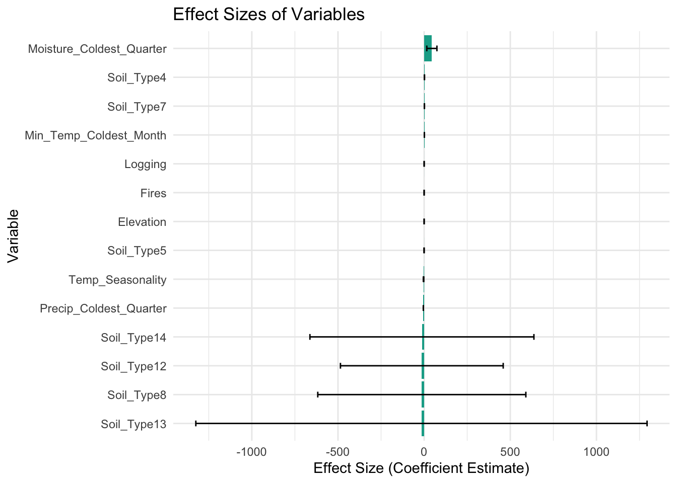
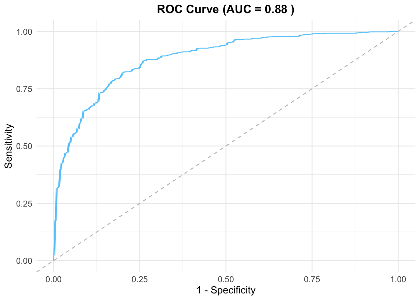
4.2 Cross validation
Now, we use the testing data to evaluate the model performance.
# Predict on the testing data
predicted_probs <- predict(glm_model, newdata = test_data, type = "response")

# Create an ROC curve and compute AUC
roc_curve <- roc(test_data$occrrnS, predicted_probs)
Setting levels: control = 0, case = 1Setting direction: controls < casesauc_value <- auc(roc_curve)
# Extract ROC data for ggplot
roc_data <- data.frame(
Sensitivity = roc_curve$sensitivities,
Specificity = 1 - roc_curve$specificities
)
# Plot the ROC curve using ggplot2
ggplot(roc_data, aes(x = Specificity, y = Sensitivity)) +
geom_line(color = "#61cafa", linewidth = 0.5) + # ROC curve
geom_abline(slope = 1, intercept = 0, linetype = "dashed", color = "gray") + # Diagonal line
labs(
title = paste("ROC Curve (AUC =", round(auc_value, 2), ")"),
x = "1 - Specificity",
y = "Sensitivity"
) +
theme_minimal() + # Minimal theme
theme(
plot.title = element_text(hjust = 0.5, size = 14, face = "bold"), # Centered and bold title
axis.title = element_text(size = 12), # Axis label font size
axis.text = element_text(size = 10) # Axis tick font size
)
plot_species_response <- function(glm_model, predictors, data) {
  # Check if required libraries are installed
  if (!requireNamespace("ggplot2", quietly = TRUE) || !requireNamespace("gridExtra", quietly = TRUE)) {
    stop("Please install the 'ggplot2' and 'gridExtra' packages to use this function.")
  }
  library(ggplot2)
  library(gridExtra)

  # Create empty list to store response plots
  response_plots <- list()

  # Loop through each predictor variable
  for (predictor in predictors) {
    # Create new data frame to vary predictor while keeping others constant
    pred_range <- seq(
      min(data[[predictor]], na.rm = TRUE),
      max(data[[predictor]], na.rm = TRUE),
      length.out = 100
    )
    const_data <- data[1, , drop = FALSE]  # Use first row to keep other predictors constant
    response_data <- const_data[rep(1, 100), ]  # Duplicate the row
    response_data[[predictor]] <- pred_range

    # Predict probabilities
    predicted_response <- predict(glm_model, newdata = response_data, type = "response")

    # Create data frame for plotting
    plot_data <- data.frame(
      Predictor_Value = pred_range,
      Predicted_Probability = predicted_response
    )

    # Add presence and absence data
    presence_absence_data <- data.frame(
      Predictor_Value = data[[predictor]],
      Presence_Absence = data$occrrnS
    )

    # Generate the response plot
    p <- ggplot() +
      geom_line(data = plot_data, aes(x = Predictor_Value, y = Predicted_Probability), color = "#61c6fa", linewidth = 1) +
      geom_point(data = presence_absence_data[presence_absence_data$Presence_Absence == 1, ], aes(x = Predictor_Value, y = Presence_Absence), color = "#11aa96", alpha = 0.6) +
      geom_point(data = presence_absence_data[presence_absence_data$Presence_Absence == 0, ], aes(x = Predictor_Value, y = Presence_Absence), color = "#f6aa70", alpha = 0.6) +
      labs(x = predictor, y = NULL) +
      theme_minimal() +
      theme(axis.title.y = element_blank())

    # Store the plot in the list
    response_plots[[predictor]] <- p
  }

  # Arrange all plots in one combined plot with a single shared y-axis label
  grid.arrange(
    grobs = response_plots,
    ncol = 3,
    left = "Predicted Probability / Presence-Absence"
  )
}

# Example usage:
predictors <- c("Temp_Seasonality", "Min_Temp_Coldest_Month", "Precip_Coldest_Quarter", "Moisture_Coldest_Quarter", "Elevation", "Fires", "Logging")
plot_species_response(glm_model, predictors, train_data)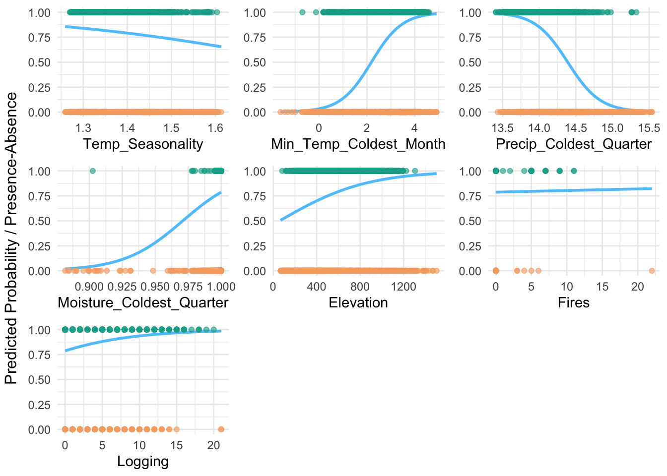
# Density and Histogram Plot Function
plot_density_histogram <- function(predicted_probs, actual_labels) {
  # Combine data into a data frame
  plot_data <- data.frame(
    Predicted_Probability = predicted_probs,
    Presence_Absence = factor(actual_labels, levels = c(0, 1), labels = c("Absence", "Presence"))
  )

  # Plot density and histogram
  ggplot(plot_data, aes(x = Predicted_Probability, fill = Presence_Absence)) +
    geom_histogram(aes(y = after_stat(density)), bins = 10, alpha = 0.6, position = "identity") +  # Histogram with density
    geom_density(alpha = 0.4) +  # Density curve
    labs(
      title = "Density and Histogram of Predicted Probabilities",
      x = "Predicted Probability",
      y = "Density",
      fill = "Presence/Absence"
    ) +
    scale_fill_manual(values = c("#f6aa70", "#11aa96")) +  # Custom colors
    theme_minimal() +
    theme(
      plot.title = element_text(hjust = 0.5, size = 14, face = "bold"),
      axis.title = element_text(size = 12),
      axis.text = element_text(size = 10),
      legend.position = "top"
    )
}

# Example usage:
# Replace `predicted_probs` with your predicted probabilities and `test_data$occrrnS` with your actual labels
plot_density_histogram(predicted_probs, test_data$occrrnS)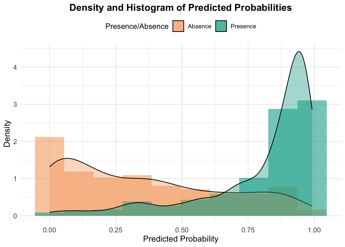
5. Mapping and Interpolation
If you remember, we started with these point records of mountain ash

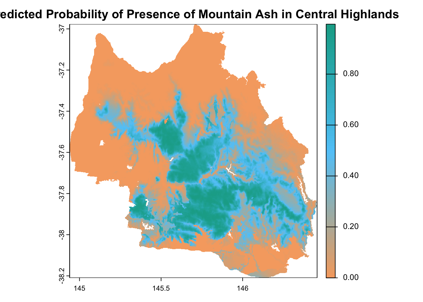
Now, let’s predict a continuous mapping of the distribution of mountain ash in the central highlands.
# Predict the presence probability across the entire raster extent
predicted_raster <- predict(env_var_stack, glm_model, type = "response")
|---------|---------|---------|---------|
=========================================
# Define a custom color palette
custom_palette <- colorRampPalette(c("#f6aa70", "#61cafa", "#11aa96"))


# Plot the raster with the custom color palette
plot(
  predicted_raster,
  main = "Predicted Probability of Presence of Mountain Ash in Central Highlands",
  col = custom_palette(100) # Use 100 colors for smooth transitions
)
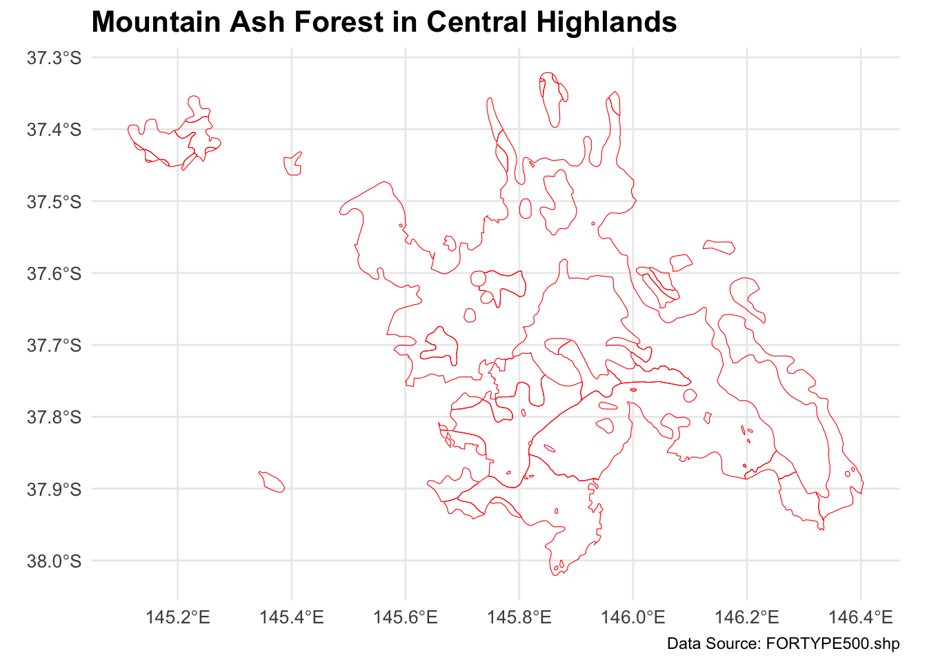
We can also use an independent mountain ash data to cross-validate your mapping.
forest_type_vic <- st_read("mountain_ash_centralhighlands/FORTYPE500.shp")Reading layer `FORTYPE500' from data source
`/Users/xiangzhaoqcif/dev/notebook-blog/notebooks/EC_GLM/mountain_ash_centralhighlands/FORTYPE500.shp'
using driver `ESRI Shapefile'
Simple feature collection with 5635 features and 4 fields
Geometry type: POLYGON
Dimension: XY
Bounding box: xmin: 140.9631 ymin: -39.23567 xmax: 149.9737 ymax: -33.99701
Geodetic CRS: GDA94forest_type_central_highlands <- st_intersection(forest_type_vic, central_highlands)Warning: attribute variables are assumed to be spatially constant throughout
all geometriesggplot(data = forest_type_central_highlands) +
geom_sf(aes(fill = as.factor(X_DESC)), color = NA) +
scale_fill_manual(
name = "Forest Type",
values = c(
"#D55E00", "#56B4E9", "#009E73", "#F0E442", "#0072B2",
"#CC79A7", "#E69F00", "#000000", "#8E44AD",
"#3498DB", "#F39C12","#27AE60", "#E74C3C", "#BDC3C7"
)
) +
labs(title = "Forest Types in the Central Highlands") +
theme_minimal() +
theme(
legend.position = "right",
legend.text = element_text(size = 8), # Smaller legend text
legend.title = element_text(size = 10), # Smaller legend title
plot.title = element_text(size = 16, face = "bold"), # Larger plot title
axis.text = element_text(size = 10), # Adjust axis text
axis.title = element_text(size = 12) # Adjust axis title
) +
coord_sf(expand = FALSE)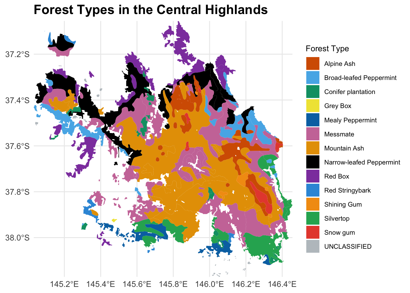
mountain_ash_forest <- forest_type_central_highlands[forest_type_central_highlands$X_DESC == "Mountain Ash", ]

# Plot the filtered shapefile
ggplot(data = mountain_ash_forest) +
  geom_sf(fill = "NA", color = "red", size = 0.1) +  # Blue fill and black border
  labs(
    title = "Mountain Ash Forest in Central Highlands",
    caption = "Data Source: FORTYPE500.shp"
  ) +
  theme_minimal() +
  theme(
    plot.title = element_text(size = 16, face = "bold"),
    axis.text = element_text(size = 10),
    axis.title = element_blank(),
    legend.position = "none"  # No legend needed since this is a single type
  )
custom_palette <- c("#f6aa70", "#61cafa", "#11aa96")


pal <- colorNumeric(
  palette = custom_palette,      # Use custom colors
  domain = values(predicted_raster),
  na.color = "transparent"       # Make NA values transparent
)

# Create the leaflet map
leaflet() %>%
  addProviderTiles(providers$Esri.WorldImagery) %>%
  # Add raster layer
  addRasterImage(predicted_raster, color = pal, opacity = 0.7, project = TRUE) %>%
  # Add shapefile layer
  addPolygons(
    data = mountain_ash_forest,
    color = "red",              # Border color of shapefile polygons
    weight = 1,                  # Border width
    fillColor = "lightblue",     # Fill color of shapefile polygons
    fillOpacity = 0.3            # Transparency for fill
  ) %>%
  # Add legend for raster
  addLegend(
    pal = pal,
    values = values(predicted_raster),
    title = "Probability",
    position = "bottomright"
  )
Warning: sf layer has inconsistent datum (+proj=longlat +ellps=GRS80 +no_defs).
Need '+proj=longlat +datum=WGS84'References
Burns, E. L., Lindenmayer, D. B., Stein, J., Blanchard, W., McBurney, L., Blair, D., & Banks, S. C. (2015). Ecosystem assessment of mountain ash forest in the C entral H ighlands of V ictoria, south‐eastern A ustralia. Austral Ecology, 40(4), 386-399.
von Takach Dukai, B. (2019). The genetic and demographic impacts of contemporary disturbance regimes in mountain ash forests.
Nevill, P. G., Bossinger, G., & Ades, P. K. (2010). Phylogeography of the world’s tallest angiosperm, Eucalyptus regnans: evidence for multiple isolated Quaternary refugia. Journal of Biogeography, 37(1), 179-192.
Zurell, D., Franklin, J., König, C., Bouchet, P. J., Dormann, C. F., Elith, J., Fandos, G., Feng, X., Guillera‐Arroita, G., & Guisan, A. (2020). A standard protocol for reporting species distribution models. Ecography, 43(9), 1261-1277.
Logging History (1930-07-01 - 2022-06-30), Data VIC, 2024, https://discover.data.vic.gov.au/dataset/logging-history-overlay-of-most-recent-harvesting-activities
Fire History (2011-2021), Data VIC, 2024, https://www.agriculture.gov.au/abares/forestsaustralia/forest-data-maps-and-tools/spatial-data/forest-fire#fires-in-australias-forests-201116-2018
Forest types of Victoria, Data VIC, 2024, https://discover.data.vic.gov.au/dataset/forest-types-of-victoria
Victory shapefile, Australian Bureau of Statistics, 2021, https://www.abs.gov.au/statistics/standards/australian-statistical-geography-standard-asgs-edition-3/jul2021-jun2026/access-and-downloads/digital-boundary-files
Harwood, Tom (2019): 9s climatology for continental Australia 1976-2005: BIOCLIM variable suite. v1. CSIRO. Data Collection. https://doi.org/10.25919/5dce30cad79a8
3 second SRTM Derived Digital Elevation Model (DEM) Version 1.0, Geoscience Australia, 2018, https://dev.ecat.ga.gov.au/geonetwork/srv/api/records/a05f7892-ef04-7506-e044-00144fdd4fa6
Searle, R. (2021): Australian Soil Classification Map. Version 1. Terrestrial Ecosystem Research Network. (Dataset). https://doi.org/10.25901/edyr-wg85
How to cite this Notebook
Singh Chandel, A. R., Zhao, X. Y., & Lopez-Marcano, S. (2024). Species Distribution Analysis - Generalised Linear Model (GLM) (Version 1.0) [Computational notebook]. Zenodo. https://doi.org/10.5281/zenodo.19551976