Automated wildlife identification from ALA camera-trap images using SpeciesNet

Author details: Dr Renuka Sharma

Editor details: Xiang Zhao

Contact details: support@ecocommons.org.au

Copyright statement: This script is the product of the EcoCommons platform. Please refer to the EcoCommons website for more details: https://www.ecocommons.org.au/

Date: July 2026

Data source: Atlas of Living Australia (ALA) | Model: SpeciesNet by Google

Script information

This notebook, developed by the EcoCommons and WildObs team, demonstrates how to automatically identify wildlife in camera-trap images by combining two open tools: the Atlas of Living Australia (ALA) and Google’s SpeciesNet model. We query ALA for camera-trap image records using the galah-python package, download a sample of images, run SpeciesNet to detect and classify the animals in each image, and visualise the predictions.

Other file formats of this notebook

Notebook	Files	Open in Colab / ARDC Jupyter	DOI
SpeciesNet

Introduction

Wildlife monitoring at scale is one of ecology’s most data-intensive challenges. Camera traps deployed across remote landscapes can accumulate thousands of images in a single survey season — far more than any team can manually review in a reasonable time. Automatically identifying the species in each photograph would free researchers to focus on analysis rather than image sorting, but doing this accurately requires a model trained on a large and diverse set of wildlife images.

This notebook shows how to combine two open tools to tackle this problem: the Atlas of Living Australia (ALA) — Australia’s national biodiversity data platform — and SpeciesNet, a deep learning model developed by Google specifically for wildlife image classification. We query ALA for camera-trap images of target species, download a sample, run SpeciesNet to automatically identify animals in each image, and then visualise the results.

Atlas of Living Australia (ALA)

The Atlas of Living Australia (ALA) is Australia’s national biodiversity data infrastructure, funded by the Australian Government through the National Collaborative Research Infrastructure Strategy (NCRIS). It provides free, online access to hundreds of millions of occurrence records aggregated from museums, herbaria, citizen-science platforms (e.g. iNaturalist), government surveys, and camera-trap deployments. Many records include field photographs — including camera-trap imagery — which makes ALA a rich source of labelled images for testing wildlife-classification models such as SpeciesNet.

For more information, visit https://www.ala.org.au/.

The galah Python package

galah is the official data-access package built by the ALA, available for both R and Python. The Python version, galah-python, lets you query and download ALA’s occurrence records, media, and taxonomic information programmatically. In this notebook we use galah to count records, retrieve camera-trap image metadata, and filter to the datasets and species of interest.

Downloading data through galah requires a registered ALA email address (free to obtain at ala.org.au). For more information, see the galah-python documentation.

Wildlife Observatory of Australia (WildObs)

The Wildlife Observatory of Australia (WildObs) is Australia’s national platform for processing and sharing wildlife camera-trap data. WildObs streamlines biodiversity monitoring by breaking down data silos and providing researchers and policymakers with consistent, high-quality data. Raw camera-trap images are processed using artificial intelligence — including MegaDetector, SpeciesNet, and bespoke regional computer-vision models — and published using the CamtrapDP data standard. The WildObs network is supported by Australia’s National Research Infrastructure: TERN supports the field observatory and standard protocols, ALA hosts the tagged image repository, and the ARDC Planet Research Data Commons (through QCIF) is building the data management and access platform. The camera-trap images used in this notebook are drawn from datasets published to ALA through this WildObs pipeline.

For more information, visit https://wildobs.org.au and https://github.com/WildObs.

Objectives

By the end of this notebook you will be able to: - retrieve camera-trap image metadata from ALA using galah-python - run automated species identification with SpeciesNet - interpret the model’s predictions and understand when to trust them

Workflow Overview

Notebook section	What happens
1 Setup	Install and import the required Python packages
2 Download WildObs data from ALA	Query ALA with `galah-python`, filter to WildObs camera-trap datasets, and download a sample of images
3 Run SpeciesNet	Load SpeciesNet and run detection, classification, and geofenced predictions on the images
4 Summary	Review results, limitations, and next steps

Note: Run cells from top to bottom in order. All required packages are installed in the Setup cell below.

1 Setup

Install the required Python packages. Run this cell once at the start of every session — packages are not persisted between sessions.

Package	Purpose
`pandas`	Organising, cleaning, and analysing tabular data
`galah-python`	Querying and downloading biodiversity records from ALA
`requests`	Retrieving image data from URLs
`speciesnet`	Running the wildlife detection and classification model
`Pillow`	Opening, resizing, and annotating images

Tip: If you see an error after installing (e.g. a version conflict), please re-run from this cell.

# Install required packages. Harmless pip DEPRECATION / [notice] build messages
# are filtered out for a cleaner log; genuine errors still show.
! pip install pandas galah-python requests speciesnet Pillow --quiet 2>&1 | grep -viE "DEPRECATION|^\[notice\]|new release of pip|To update, run" || true

Import standard libraries and define a utility function used later to manage the image download folder. SpeciesNet-specific imports are deferred to the Run SpeciesNet section so that this cell runs quickly even before the model weights are downloaded.

import os
import time
import math
import pickle
import shutil
from pathlib import Path

import pandas as pd
import requests
import matplotlib.pyplot as plt
from PIL import Image


def empty_directory(directory: Path):
    """Delete all files and sub-directories inside *directory* without
    removing the directory itself.  Creates it if it does not yet exist."""
    if not directory.exists():
        directory.mkdir(parents=True)
        return
    for item in directory.iterdir():
        if item.is_file() or item.is_symlink():
            item.unlink()
        elif item.is_dir():
            shutil.rmtree(item)

2 Download WildObs data from ALA

The Atlas of Living Australia (ALA) is Australia’s national biodiversity data infrastructure, aggregating over 130 million occurrence records from museums, herbaria, citizen science platforms (e.g. iNaturalist), and government surveys. Many of these records include photographs taken in the field — including images from camera-trap deployments — which is exactly what we need to test SpeciesNet.

We use the galah-python package to query ALA’s API and retrieve image metadata for our target species.

2.1 Configure galah

galah requires a registered ALA email address to submit download requests. Registration is free at ala.org.au. Replace the placeholder email below with your own. You can also change the taxa list to any species you are interested in — use the scientific (Latin) name.

import os
import galah

# Replace with your own ALA-registered email, or set the ALA_EMAIL environment
# variable before running. Registration is free at https://www.ala.org.au/
galah.galah_config(
    atlas="Australia",
    email=os.environ.get("ALA_EMAIL", "your-email@example.com"),
)
print("galah config applied.")

# Species to query — use scientific (Latin) names
# You can add or remove species from this list, keep it under 3 for ease of processing at this stage
# taxa = ['Felis catus', 'Sus scrofa', 'Canis dingo']
taxa = ['Felis catus', 'Sus scrofa']

print(f"\nQuerying {len(taxa)} species:")
for i, sp in enumerate(taxa, 1):
    print(f"  {i}. {sp}")

galah config applied.

Querying 2 species:
  1. Felis catus
  2. Sus scrofa

2.2 Check record counts

Before fetching full metadata, it is worth checking how many image records exist for your taxa and geographic filter. This is a fast call that does not trigger a download — it gives you a sense of dataset size so you can decide whether to narrow your filters further. The cell below returns a count broken down by media type.

galah.atlas_counts(
    taxa=taxa,
    filters=['stateProvince=Queensland'],
    group_by="multimedia"
)

	multimedia	count
0	Image	3349

2.3 Fetch image metadata

Now we retrieve the full image metadata using galah.atlas_media(). This returns a table of records that includes the image URL, species name, data-resource name, and observation coordinates for every matching record. Crucially, setting collect=False means we are only downloading the metadata — not the image files themselves, which we will do in a later step.

This call submits a download job to ALA’s servers and polls until it is ready, which can take anywhere from under a minute to well over ten minutes depending on how many records match your filters. Adding year and month filters (as below) significantly reduces the wait time — as a reference point, filtering to a single Australian state, year, and month typically completes in two to three minutes.

Note for Google Colab users: ALA’s download service occasionally blocks requests from cloud provider IP addresses, returning a JSONDecodeError or 403 Forbidden. If you encounter this, try re-running the cell. If it persists, run this cell locally, save the result with media_df.to_csv("media_df.csv"), then upload that file to Colab and load it with media_df = pd.read_csv("media_df.csv").

media_df = galah.atlas_media(
    taxa=taxa,
    filters=["stateProvince=Queensland", "year=2023", "month=1"],  # narrow filters = faster
    multimedia="images",
    collect=False,   # metadata only — image files are NOT downloaded here
)

print(f"Retrieved {len(media_df)} image records.")
media_df.head()

Retrieved 984 image records.

	decimalLatitude	decimalLongitude	eventDate	scientificName	recordID	dataResourceName	occurrenceStatus	multimedia	images	videos	sounds	creator	license	mimetype	width	height	imageUrl
0	-25.646330	152.648088	2023-01-20T11:03:00Z	Sus scrofa	c1927840-53ff-4669-b205-ba3236411881	iNaturalist Australia	PRESENT	Image	26ccaec7-1f97-457d-aaf0-9a0b04c66629	NaN	NaN	Scott W. Gavins	http://creativecommons.org/licenses/by-nc/4.0/	image/jpeg	2048	1536	https://images.ala.org.au/store/9/2/6/6/26ccae...
1	-17.289829	145.795254	2023-01-27T00:00:00Z	Sus scrofa	e0dbce7e-ccf0-45ea-8293-0ab9ac4155c0	Camera trap surveys in Queensland's Wet Tropic...	PRESENT	Image	b6d29931-1065-4e18-839c-bbbcee13d632	NaN	NaN	None	None	image/jpeg	5376	3024	https://images.ala.org.au/store/2/3/6/d/b6d299...
2	-17.289829	145.795254	2023-01-01T00:00:00Z	Sus scrofa	d21a13ec-a189-44fd-aa5d-2267ce9ec962	Camera trap surveys in Queensland's Wet Tropic...	PRESENT	Image	4496b905-1199-40d0-8817-8170487d2693	NaN	NaN	None	None	image/jpeg	5376	3024	https://images.ala.org.au/store/3/9/6/2/4496b9...
3	-17.289829	145.795254	2023-01-06T00:00:00Z	Sus scrofa	4d222fde-90ff-4387-b38d-ce696dc6cf46	Camera trap surveys in Queensland's Wet Tropic...	PRESENT	Image	2e14e786-8fbe-43e4-a4e3-088dc16af8f1	NaN	NaN	None	None	image/jpeg	5376	3024	https://images.ala.org.au/store/1/f/8/f/2e14e7...
4	-17.289829	145.795254	2023-01-27T00:00:00Z	Sus scrofa	a58133e1-e5c3-47a6-8eac-5542821ef28f	Camera trap surveys in Queensland's Wet Tropic...	PRESENT	Image	7d94d39b-0f7c-4c62-8f65-33cdc3d08831	NaN	NaN	None	None	image/jpeg	5376	3024	https://images.ala.org.au/store/1/3/8/8/7d94d3...

2.4 Inspect the data

Before filtering, take a look at what data resources and species came back. ALA aggregates records from many different providers, and the quality and type of images varies considerably between them. Knowing which datasets are present lets you make an informed decision about which ones to keep.

print("Columns:", media_df.columns.tolist())
print("\nUnique data resources:")
for dr in media_df['dataResourceName'].unique():
    print(" •", dr)
print("\nUnique scientific names:")
for sp in media_df['scientificName'].unique():
    print(" •", sp)

Columns: ['decimalLatitude', 'decimalLongitude', 'eventDate', 'scientificName', 'recordID', 'dataResourceName', 'occurrenceStatus', 'multimedia', 'images', 'videos', 'sounds', 'creator', 'license', 'mimetype', 'width', 'height', 'imageUrl']

Unique data resources:
 • iNaturalist Australia
 • Camera trap surveys in Queensland's Wet Tropics 2022-2023

Unique scientific names:
 • Sus scrofa
 • Felis catus

2.5 Filter to camera-trap datasets

Not all ALA image records are equally suitable for SpeciesNet. The model was trained on camera-trap images and performs best on that type of photograph. Field photos, museum specimens, or heavily cropped images can produce unreliable predictions. Here we restrict the data to records from the Wildlife Observatories of Australia (WildObs) dataset, which contains high-quality, labelled camera-trap images, and keep only the target species of interest.

Update values_to_keep with the dataset names you saw in the previous cell, and adjust target_species to match your taxa of interest.

values_to_keep = [
    "Camera trap surveys in Queensland's Wet Tropics 2022-2023",
    "Monitoring many landscapes in VIC-NSW border to assess impacts of 2019-20 gigafires on wildlife diel activity",
    "Wombat burrows are hotspots for small vertebrates in a landscape subject to gigafire",
]
target_species = ['Felis catus', 'Sus scrofa', 'Canis dingo']

filtered_df = media_df[
    media_df["dataResourceName"].isin(values_to_keep) &
    media_df["scientificName"].isin(target_species)
]

print(f"Records after filtering: {len(filtered_df)}")
filtered_df.head()

Records after filtering: 981

	decimalLatitude	decimalLongitude	eventDate	scientificName	recordID	dataResourceName	occurrenceStatus	multimedia	images	videos	sounds	creator	license	mimetype	width	height	imageUrl
1	-17.289829	145.795254	2023-01-27T00:00:00Z	Sus scrofa	e0dbce7e-ccf0-45ea-8293-0ab9ac4155c0	Camera trap surveys in Queensland's Wet Tropic...	PRESENT	Image	b6d29931-1065-4e18-839c-bbbcee13d632	NaN	NaN	None	None	image/jpeg	5376	3024	https://images.ala.org.au/store/2/3/6/d/b6d299...
2	-17.289829	145.795254	2023-01-01T00:00:00Z	Sus scrofa	d21a13ec-a189-44fd-aa5d-2267ce9ec962	Camera trap surveys in Queensland's Wet Tropic...	PRESENT	Image	4496b905-1199-40d0-8817-8170487d2693	NaN	NaN	None	None	image/jpeg	5376	3024	https://images.ala.org.au/store/3/9/6/2/4496b9...
3	-17.289829	145.795254	2023-01-06T00:00:00Z	Sus scrofa	4d222fde-90ff-4387-b38d-ce696dc6cf46	Camera trap surveys in Queensland's Wet Tropic...	PRESENT	Image	2e14e786-8fbe-43e4-a4e3-088dc16af8f1	NaN	NaN	None	None	image/jpeg	5376	3024	https://images.ala.org.au/store/1/f/8/f/2e14e7...
4	-17.289829	145.795254	2023-01-27T00:00:00Z	Sus scrofa	a58133e1-e5c3-47a6-8eac-5542821ef28f	Camera trap surveys in Queensland's Wet Tropic...	PRESENT	Image	7d94d39b-0f7c-4c62-8f65-33cdc3d08831	NaN	NaN	None	None	image/jpeg	5376	3024	https://images.ala.org.au/store/1/3/8/8/7d94d3...
5	-17.289829	145.795254	2023-01-07T00:00:00Z	Sus scrofa	8ac2d718-dbf8-49d9-b067-08584289ea2a	Camera trap surveys in Queensland's Wet Tropic...	PRESENT	Image	97918c43-22e0-458d-bebd-48d3292515a0	NaN	NaN	None	None	image/jpeg	5376	3024	https://images.ala.org.au/store/0/a/5/1/97918c...

2.6 Select a sample

Running SpeciesNet on hundreds of images can take a long time, especially without a GPU. For now, we randomly select a small subset to keep things manageable. Once you are comfortable with the workflow, you can increase N_IMAGES or remove the sampling step entirely to process the full filtered dataset. Setting random_state=42 ensures the same images are chosen every time you run the cell, which is useful for reproducibility.

N_IMAGES = 6  # number of images to download

subset_df = filtered_df.sample(min(N_IMAGES, len(filtered_df)), random_state=42)
print(f"Subset size: {len(subset_df)}")
subset_df[["scientificName", "dataResourceName", "imageUrl"]].reset_index(drop=True)

Subset size: 6

	scientificName	dataResourceName	imageUrl
0	Felis catus	Camera trap surveys in Queensland's Wet Tropic...	https://images.ala.org.au/store/b/a/e/c/696946...
1	Sus scrofa	Camera trap surveys in Queensland's Wet Tropic...	https://images.ala.org.au/store/5/e/2/5/8b95d6...
2	Sus scrofa	Camera trap surveys in Queensland's Wet Tropic...	https://images.ala.org.au/store/6/7/0/0/7ac65b...
3	Sus scrofa	Camera trap surveys in Queensland's Wet Tropic...	https://images.ala.org.au/store/a/3/3/b/ab0f5c...
4	Sus scrofa	Camera trap surveys in Queensland's Wet Tropic...	https://images.ala.org.au/store/2/a/2/0/3514bf...
5	Felis catus	Camera trap surveys in Queensland's Wet Tropic...	https://images.ala.org.au/store/5/2/2/5/9313e1...

2.7 Download images

Now we download the actual image files from their ALA-hosted URLs and save them to the EC_images folder. The folder is cleared at the start of each run so that images from a previous run do not accumulate. Each file is named after its DataFrame row index (e.g. 144.jpg), making it straightforward to trace a prediction back to the original metadata record.

image_folder = Path("EC_images")
empty_directory(image_folder)   # clears the folder (or creates it if new)

for i, row in subset_df.iterrows():
    url = row["imageUrl"]
    filename = image_folder / f"{i}.jpg"
    try:
        r = requests.get(url, timeout=30)
        r.raise_for_status()
        filename.write_bytes(r.content)
        print(f"Downloaded: {filename.name}")
    except Exception as e:
        print(f"Failed to download {url}: {e}")

print(f"\nDone. {len(list(image_folder.glob('*.jpg')))} images saved to '{image_folder}'.")

Downloaded: 792.jpg
Downloaded: 498.jpg
Downloaded: 140.jpg
Downloaded: 571.jpg
Downloaded: 67.jpg
Downloaded: 762.jpg

Done. 6 images saved to 'EC_images'.

2.8 Preview the images

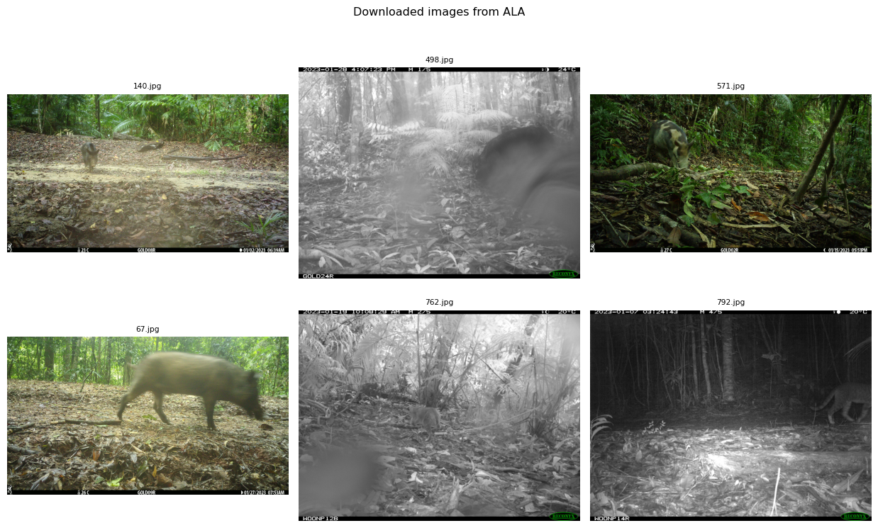
Before running the model, display the downloaded images as a grid to confirm they look as expected. This is a good moment to spot any blank frames, setup photos, or corrupted files that might produce unreliable predictions and should be excluded before analysis.

image_paths = sorted(image_folder.glob("*.jpg"))
print(f"Found {len(image_paths)} images.")

n_show = min(6, len(image_paths))
fig, axes = plt.subplots(2, 3, figsize=(13, 8))

for ax, img_path in zip(axes.flatten(), image_paths[:n_show]):
    img = Image.open(img_path)
    ax.imshow(img)
    ax.set_title(img_path.name, fontsize=8)
    ax.axis("off")

# Hide unused subplot panels
for ax in axes.flatten()[n_show:]:
    ax.set_visible(False)

plt.suptitle("Downloaded images from ALA", fontsize=12, y=1.01)
plt.tight_layout()
plt.show()

Found 6 images.

3 Run SpeciesNet

SpeciesNet is a deep learning model developed by Google for automated wildlife identification in camera-trap images. It was trained on over 65 million camera-trap images from the Wildlife Insights platform, making it one of the most extensively trained wildlife classifiers available.

The model works in two stages. First, a detector scans the image and draws a bounding box around any animal it finds, along with a confidence score (0–1) indicating how certain it is that an animal is present. Second, a classifier examines the content inside the bounding box — or the full image if no box was found — and assigns the most likely species label from a vocabulary of over 2,000 labels. These labels span individual species (e.g. Sus scrofa, wild boar), broader taxonomic groups (e.g. "felidae", cat family), and non-animal classes ("blank", "vehicle", "human").

3.1 Geofencing

SpeciesNet includes a geofencing step that filters out predictions for species known not to occur in a given country. For example, if you supply country="AUS", the model will not predict “lion” or “elephant” for an Australian image, even if the raw classifier score for those labels is high. Geofencing is enabled by default and is strongly recommended whenever you are working within a defined geographic region — it meaningfully reduces false positives.

3.2 Load libraries

Import the SpeciesNet library and define a small helper function that prints predictions in a readable format. We also print the available models — DEFAULT_MODEL is the recommended choice for most use cases.

import warnings
warnings.filterwarnings('ignore')

from IPython.display import display, JSON

from speciesnet import DEFAULT_MODEL, SUPPORTED_MODELS
from speciesnet import draw_bboxes, load_rgb_image, SpeciesNet


def print_predictions(predictions_dict: dict) -> None:
    """Print a human-readable summary of SpeciesNet predictions."""
    print("Predictions:")
    for pred in predictions_dict["predictions"]:
        print(f"  {Path(pred['filepath']).name}  =>  {pred['prediction']}")


print("Default model :", DEFAULT_MODEL)
print("Supported models:", SUPPORTED_MODELS)

Default model : kaggle:google/speciesnet/pyTorch/v4.0.3a/1
Supported models: ['kaggle:google/speciesnet/pyTorch/v4.0.3a/1', 'kaggle:google/speciesnet/pyTorch/v4.0.3b/1']

3.3 Load the model

The cell below loads SpeciesNet. The first time it runs, it will download the model weights (approximately 1–2 GB), which can take a few minutes. Subsequent runs in the same session use the cached weights instantly.

Tip for Colab users: Colab’s local disk is wiped when the runtime disconnects, so the weights will need to be re-downloaded each session. To avoid this, mount your Google Drive and point the cache there:
from google.colab import drive
drive.mount('/content/drive')
model = SpeciesNet(DEFAULT_MODEL, cache_dir="/content/drive/MyDrive/speciesnet_cache")

model = SpeciesNet(DEFAULT_MODEL)          # geofencing ON  (default)
# model = SpeciesNet(DEFAULT_MODEL, geofence=False)  # uncomment to disable geofencing
print("Model loaded.")

Model loaded.

3.4 Run predictions

Pass the image folder to model.predict(). SpeciesNet will find every .jpg, .jpeg, and .png file in the folder, run the detector and classifier on each one, and return a dictionary of results — one entry per image.

predictions_dict = model.predict(folders=[image_folder])
print_predictions(predictions_dict)
# display(JSON(predictions_dict))  # uncomment for the full verbose output

Predictions:
  140.jpg  =>  d372cda5-a8ca-4b7b-97ed-4e4fab9c9b4b;mammalia;artiodactyla;suidae;sus;scrofa;wild boar
  498.jpg  =>  988b8b2d-6d3b-4c5f-899c-c76b6108b90b;mammalia;artiodactyla;tayassuidae;;;peccary family
  571.jpg  =>  d372cda5-a8ca-4b7b-97ed-4e4fab9c9b4b;mammalia;artiodactyla;suidae;sus;scrofa;wild boar
  67.jpg  =>  d372cda5-a8ca-4b7b-97ed-4e4fab9c9b4b;mammalia;artiodactyla;suidae;sus;scrofa;wild boar
  762.jpg  =>  9212982e-8a58-4775-a6ac-e9a43110d8f5;mammalia;carnivora;felidae;felis;catus;domestic cat
  792.jpg  =>  9212982e-8a58-4775-a6ac-e9a43110d8f5;mammalia;carnivora;felidae;felis;catus;domestic cat

How to read a prediction string:

Each prediction is a semicolon-separated string with 7 fields:

1b30ddf8-22fb-40ff-9df6-6a8a0b6ccaa1 ; mammalia ; monotremata ; tachyglossidae ; tachyglossus ; aculeatus ; short-beaked echidna

UUID; Class; Order; Family; Genus; Species; Common name

UUID — unique label identifier in the SpeciesNet taxonomy
Class → Species — full taxonomic hierarchy from class down to species epithet
Common name — plain-language species name (last field, easiest to read)

If the model is not confident about a species, it may predict at a higher taxonomic level (e.g. "felidae;;; cat family" with blank genus/species fields).

3.5 Run on specific files

Instead of a whole folder, you can pass a list of specific file paths. This is useful when you want to quickly test the model on a single image or a hand-picked selection without re-processing the entire folder.

image_paths = sorted(
    p for p in image_folder.iterdir()
    if p.suffix.lower() in [".jpg", ".jpeg", ".png"]
)

predictions_dict = model.predict(filepaths=[image_paths[0], image_paths[1]])
print_predictions(predictions_dict)

Predictions:
  140.jpg  =>  d372cda5-a8ca-4b7b-97ed-4e4fab9c9b4b;mammalia;artiodactyla;suidae;sus;scrofa;wild boar
  498.jpg  =>  988b8b2d-6d3b-4c5f-899c-c76b6108b90b;mammalia;artiodactyla;tayassuidae;;;peccary family

3.6 Visualise results

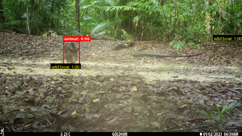
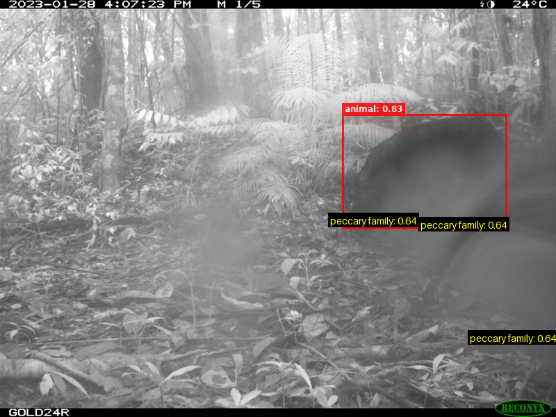
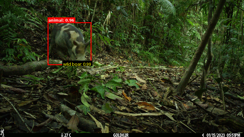
The cell below displays each image with its predictions overlaid. Where the detector found an animal, a red bounding box is drawn around it. The detector’s confidence score appears in the top-left corner of the box (e.g. animal: 0.88), and the classifier’s species label with its confidence score is shown in the bottom-right corner (e.g. domestic cat: 0.93). The exact labels and scores you see will depend on your images and taxa.

Where the detector found nothing — which can happen with blurry, fast-moving, or partially visible animals — the classifier’s prediction is shown as a banner at the bottom of the image. The classifier still runs on the full image in these cases, so a species label is always produced.

from PIL import ImageDraw, ImageFont

# Run SpeciesNet on all images in the folder
predictions_dict = model.predict(folders=[image_folder])

# Load a font 
font = ImageFont.load_default(size=14)  

n_show = min(3, len(predictions_dict["predictions"]))
for pred_item in predictions_dict["predictions"][:n_show]:
    fname      = Path(pred_item["filepath"]).name
    pred_text  = pred_item.get("prediction", "")
    detections = pred_item.get("detections", [])

    # The prediction string is semicolon-separated:
    # UUID ; class ; order ; family ; genus ; species ; common-name
    species_name = pred_text.split(";")[-1] if pred_text else "unknown"

    # Classifier confidence: classifications = {"classes": [...], "scores": [...]}
    # scores[0] is the top prediction's confidence (0–1)
    scores = pred_item.get("classifications", {}).get("scores", [])
    conf   = scores[0] if scores else None
    species_label = f"{species_name}: {conf:.2f}" if conf is not None else species_name

    print(f"File      : {fname}")
    print(f"Prediction: {pred_text}")

    img = load_rgb_image(pred_item["filepath"])
    img.thumbnail(size=(800, 800))

    if detections:
        # draw_bboxes draws a red box + "animal: conf" label for each detection.
        # It returns a NEW annotated image — the return value must be captured.
        img = draw_bboxes(img, detections)

        # Overlay the classifier's species label at the bottom-right of each box
        draw = ImageDraw.Draw(img)
        for det in detections:
            xmin, ymin, bw, bh = det["bbox"]
            x_right  = int((xmin + bw) * img.width)
            y_bottom = int((ymin + bh) * img.height)

            x1, y1, x2, y2 = draw.textbbox((0, 0), species_label, font=font)
            x_px = x_right  - (x2 - x1)   # right-align to box edge
            y_px = y_bottom - (y2 - y1)    # bottom-align to box edge

            draw.rectangle([x_px - 3, y_px - 3, x_right + 3, y_bottom + 3], fill=(0, 0, 0))
            draw.text((x_px, y_px), species_label, fill=(255, 255, 0), font=font)

        print(f"  {len(detections)} bounding box(es) drawn.")
    else:
        # No detection: the animal was not located above the detector's confidence
        # threshold (common with motion blur or partially visible subjects).
        # Draw the classifier result as a banner at the bottom of the image.
        draw = ImageDraw.Draw(img)
        w, h = img.size
        banner = f"Classifier: {species_label}  (no detection bbox)"
        draw.rectangle([0, h - 30, w, h], fill=(0, 0, 0))
        draw.text((6, h - 24), banner, fill=(255, 255, 255), font=font)
        print("  No bounding boxes — classifier label shown as banner.")

    print()
    display(img)

File      : 140.jpg
Prediction: d372cda5-a8ca-4b7b-97ed-4e4fab9c9b4b;mammalia;artiodactyla;suidae;sus;scrofa;wild boar
  2 bounding box(es) drawn.

File      : 498.jpg
Prediction: 988b8b2d-6d3b-4c5f-899c-c76b6108b90b;mammalia;artiodactyla;tayassuidae;;;peccary family
  3 bounding box(es) drawn.

File      : 571.jpg
Prediction: d372cda5-a8ca-4b7b-97ed-4e4fab9c9b4b;mammalia;artiodactyla;suidae;sus;scrofa;wild boar
  1 bounding box(es) drawn.

3.7 Interpreting the results

Confidence scores represent how certain the model is about a prediction, on a scale of 0 to 1. A score of 0.93 means the model assigns 93% of its probability mass to that label. As a rough guide: - > 0.9 — high confidence; likely a reliable prediction - 0.6–0.9 — moderate confidence; worth a visual check - < 0.6 — low confidence; treat with caution

When the model is uncertain at the species level, it often predicts at a higher taxonomic rank instead — for example, predicting the order "cetartiodactyla" rather than Sus scrofa. This is a deliberate and sensible fallback: a broad but correct label is more useful than a confident but wrong species name.

3.7.1 Understanding the range of predictions you may see

Even when all images in a batch share the same ALA species label, SpeciesNet may return a spread of different predictions. For example, a set of Sus scrofa (wild boar) images might yield species-level labels such as wild boar, domestic cattle, or bearded pig, alongside higher-rank predictions like Cetartiodactyla (order) or mammal (class). Your results will vary depending on which species you query and the quality of the images retrieved.

Species-level mismatches like these often reflect genuine visual ambiguity rather than random error. Animals within the same family or order — for instance, wild boar, bearded pig (Sus barbatus), and domestic cattle (Bos taurus) — all belong to Cetartiodactyla (even-toed ungulates) and can look strikingly similar in a camera-trap photograph, especially when the image is blurry, partially obstructed, or taken in low light at night.

Higher-rank predictions — such as an order or class label instead of a species name — indicate that the model could not confidently distinguish between species in that group and chose to abstain from a species-level call. This is a deliberate design choice: returning a broad but correct label (e.g. "cetartiodactyla") is more useful than a confident but wrong species name.

Taken together, this range of outputs illustrates an important point: SpeciesNet’s predictions should be treated as a probabilistic first-pass label, not a definitive identification. Predictions below ~0.9 confidence, or those returned at a higher taxonomic level than species, are best treated as candidates for expert validation or a second-pass review.

3.7.2 Known limitations

Image quality matters. SpeciesNet was trained on camera-trap images and performs best on those. Images taken at night, in heavy rain, or with severe motion blur will produce lower-confidence and less reliable predictions.
The detector and classifier are independent. The detector can miss an animal and still have the classifier produce a correct species label — and vice versa. Always look at both the bounding box and the prediction string together.
Closely related species are harder to distinguish. Species within the same family or order (e.g. Sus scrofa vs Sus barbatus) are more likely to be confused with each other than with distantly related animals, because they share similar body shapes and colouring.
“Blank” predictions are useful. If SpeciesNet predicts blank, neither the detector nor the classifier found strong evidence of an animal — valuable for automatically filtering empty frames from large datasets.
Geofencing can suppress correct predictions. If a species is present but outside its expected geographic range (e.g. an escaped or introduced animal), geofencing may filter it out. Disable it with geofence=False in those cases.

3.8 Run the classifier only

SpeciesNet’s detector and classifier can be called independently. model.classify() runs only the classifier on the full image, skipping detection entirely. This is faster and still produces a species label, but gives no information about where the animal is located in the frame. It is useful for large-scale screening where location is not needed.

# Classifier only — no bounding boxes, just species labels for the full image
predictions_dict = model.classify(filepaths=[image_paths[0], image_paths[1]])

print("Classifier-only results (top prediction per image):")
for pred in predictions_dict["predictions"]:
    fname  = Path(pred["filepath"]).name
    label  = pred.get("prediction", "").split(";")[-1]
    scores = pred.get("classifications", {}).get("scores", [])
    conf   = f"{scores[0]:.2f}" if scores else "n/a"
    print(f"  {fname}  =>  {label}  (confidence: {conf})")

# Uncomment to see the full raw output including all candidate classifications:
# display(JSON(predictions_dict))

Classifier-only results (top prediction per image):
  140.jpg  =>    (confidence: 0.56)
  498.jpg  =>    (confidence: 0.92)

3.9 Run the detector only

model.detect() runs only the detector. It returns bounding boxes and confidence scores for any animals found, but does not identify the species — each detection is simply labelled "animal". This is useful for quickly checking occupancy (is an animal present?) or filtering blank frames, without the computational overhead of species classification.

# Detector only — returns bounding boxes with confidence scores, no species labels
predictions_dict = model.detect(filepaths=[image_paths[0], image_paths[1]])

print("Detector-only results (bounding boxes per image):")
for pred in predictions_dict["predictions"]:
    fname      = Path(pred["filepath"]).name
    detections = pred.get("detections", [])
    if detections:
        for d in detections:
            print(f"  {fname}  =>  {d['label']}  conf: {d['conf']:.2f}  bbox: {d['bbox']}")
    else:
        print(f"  {fname}  =>  no detections above threshold")

# Uncomment to see the full raw output:
# display(JSON(predictions_dict))

Detector-only results (bounding boxes per image):
  140.jpg  =>  animal  conf: 0.96  bbox: [0.2613467387855053, 0.30291004478931427, 0.0682663694024086, 0.19708994030952454]
  140.jpg  =>  animal  conf: 0.04  bbox: [0.9730282882228494, 0.20568782463669777, 0.02697172574698925, 0.08366402238607407]
  498.jpg  =>  animal  conf: 0.83  bbox: [0.61572265625, 0.2740885317325592, 0.29638671875, 0.275390625]
  498.jpg  =>  animal  conf: 0.04  bbox: [0.61474609375, 0.305989570915699, 0.13427734375, 0.2330729216337204]
  498.jpg  =>  animal  conf: 0.02  bbox: [0.66064453125, 0.3098958432674408, 0.33935546875, 0.5110676884651184]

3.10 Run with geofencing

To explicitly activate geofencing with a country code, pass an instances_dict to model.predict(). Each entry in the "instances" list is a dict with a "filepath" and a "country" key. SpeciesNet uses ISO 3166-1 alpha-3 three-letter codes (case-insensitive):

Country	Code	Country	Code
Australia	`AUS`	South Africa	`ZAF`
New Zealand	`NZL`	Kenya	`KEN`
United States	`USA`	India	`IND`
Canada	`CAN`	Brazil	`BRA`
United Kingdom	`GBR`	Indonesia	`IDN`

Supplying a country code is strongly recommended when working with a known study region — it meaningfully reduces false positives for species that could not plausibly occur there.

predictions_dict = model.predict(
    instances_dict={
        "instances": [
            {"filepath": str(image_paths[1]), "country": "AUS"},
        ]
    }
)
print_predictions(predictions_dict)

Predictions:
  498.jpg  =>  a27d3983-76a1-4d2d-b080-18747cd77dcb;mammalia;artiodactyla;;;;artiodactyla order

To disable geofencing entirely (e.g. for global datasets or to see unfiltered raw predictions), reload the model with geofence=False:

model_no_geo = SpeciesNet(DEFAULT_MODEL, geofence=False)
predictions_dict = model_no_geo.predict(folders=[image_folder])

When to disable geofencing: Useful if you are working with images from multiple countries in a single batch, or if you want to inspect the model’s raw confidence scores before geographic filtering.

4 Summary

This notebook has shown how to combine two open tools — ALA’s biodiversity data platform and Google’s SpeciesNet model — to automatically identify animal species in camera-trap images. Starting from a simple species query, we retrieved image records from ALA, downloaded a sample, and ran SpeciesNet to produce species labels and bounding boxes for each photograph.

Automated image classification won’t replace expert review for all use cases, but it can dramatically reduce the manual effort involved in processing large camera-trap datasets — particularly for filtering blank frames, flagging images likely to contain a species of interest, or generating a first-pass label for subsequent expert validation.

To take this further, try: - replacing the taxa or geographic filter to work with a different study system - increasing N_IMAGES to run the model on your full filtered dataset - exporting predictions to a CSV with pd.DataFrame(predictions_dict["predictions"]).to_csv("results.csv") - joining predictions back to subset_df on the image filename to add location, date, and data-resource context

Resources: - galah-python documentation - SpeciesNet GitHub repository - Atlas of Living Australia - EcoCommons notebooks

References

Atlas of Living Australia (2026). Occurrence and multimedia records. Atlas of Living Australia. Available at: https://www.ala.org.au/ (Accessed: 16 July 2026).

Westgate, M., Kellie, D., Stevenson, M., & Newman, P. galah: Biodiversity Data from the Atlas of Living Australia and the GBIF Node Network. Python package. Documentation: https://galah.ala.org.au/Python/

Google LLC (2024). SpeciesNet: Deep learning models for identifying animals in camera-trap imagery (cameratrapai). GitHub repository (Apache License 2.0). https://github.com/google/cameratrapai

How to cite this Notebook

Sharma, R., & Zhao, X. Y. (2026). Automated wildlife identification from ALA camera-trap images using SpeciesNet (Version 1.0) [Computational notebook]. Zenodo. https://doi.org/10.5281/zenodo.21522834

Copyright information from SpeciesNet

Licensed under the Apache License, Version 2.0 (the “License”); you may not use this file except in compliance with the License. You may obtain a copy of the License at

https://www.apache.org/licenses/LICENSE-2.0

Unless required by applicable law or agreed to in writing, software distributed under the License is distributed on an “AS IS” BASIS, WITHOUT WARRANTIES OR CONDITIONS OF ANY KIND, either express or implied. See the License for the specific language governing permissions and limitations under the License.