Species Distribution Modelling - Random Forest

Author details: Xiang Zhao

Editor details: Dr Jenna Wraith

Contact details: support@ecocommons.org.au

Copyright statement: This script is the product of the EcoCommons platform. Please refer to the EcoCommons website for more details: https://www.ecocommons.org.au/

Date: May 2025

Script information

This notebook, developed by the EcoCommons team, showcases how to build Species Distribution Models (SDMs) using Random Forest algorithm. It also compares the SDMs generated for the same species using Random Forest and Generalised Linear Models, highlighting their differences in predictive performance and spatial output.

Introduction

Using Mountain Ash (Eucalyptus regnans), a very tall and straight tree species native to Victoria and Tasmania, we will guide you through a standard protocol developed by Zurell et al. (2020) for building species distribution models (SDMs) with one of the most widely used algorithms: the Random Forest (RF). We will also demonstrate the performance differences of SDMs produced by Random Forest algorithm and Generalised Linear Model (GLM) algorithm.

Key concepts

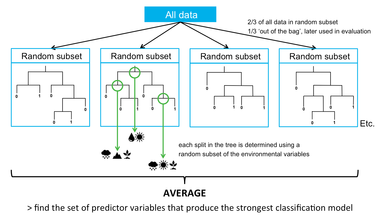
K.1 Random forests

Random Forests are an extension of single Classification Trees in which multiple decision trees are built with random subsets of the data. All random subsets have the same number of data points, and are selected from the complete dataset. Used data is placed back in the full dataset and can be selected in subsequent trees. In Random Forests, the random subsets are selected in a procedure called ‘bagging’, in which each data point has an equal probability of being selected for each new random subset. About two thirds of the total dataset is included in each random subset. The other third of the data is not used to build the trees, and this part is called the ‘out-of-the-bag’ data. This part is later used to evaluate the model.

K.2 Decision tree

Each single classification tree is a decision tree. A decision tree is a predictive model that makes decisions by splitting data into branches based on if-then rules.

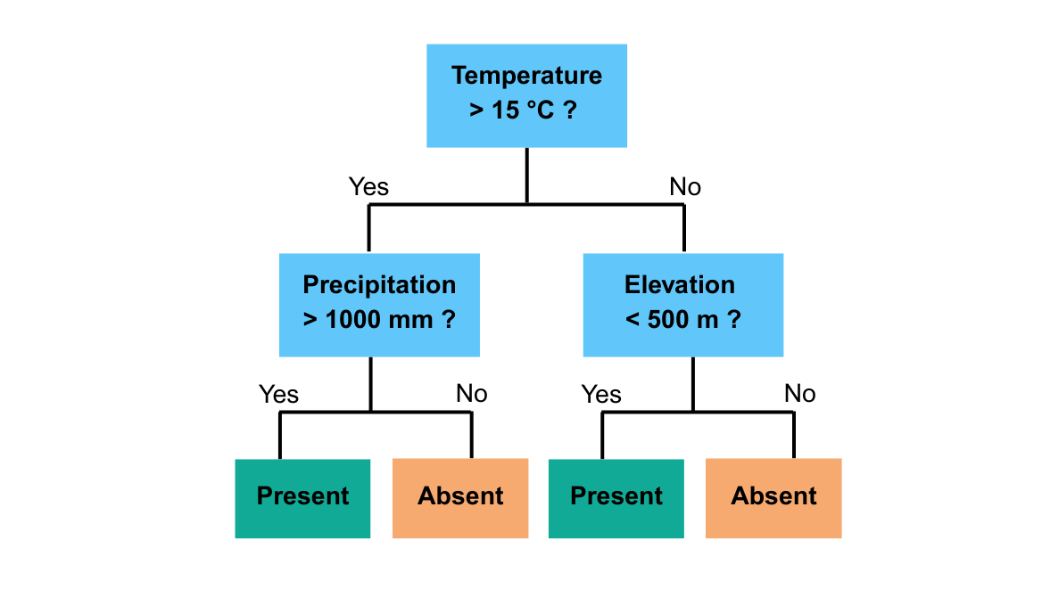
For example, the above decision tree means:

If temperature > 15°C and precipitation > 1000 mm then predict species present
If temperature > 15°C but precipitation ≤ 1000 mm then predict absent
If temperature ≤ 15°C and elevation < 500 m then predict absent
If temperature ≤ 15°C and elevation ≥ 500 m then predict present

This is a small decision tree that splits the landscape into four groups using three environmental variables. A real random forest would grow many of these, each on a random subset of data and predictors, and combine their results.

K.3 Bootstrap sampling and out-of-bag (OOB)

A bootstrap sampling means random sampling with replacement. When Random Forest builds each decision tree, it randomly selects a subset of the data from the original dataset. The subset is the same size as the original dataset. But some rows are repeated and some are left out.

The out-of-bag data are the observations that were not included in the bootstrap sample for a particular tree.

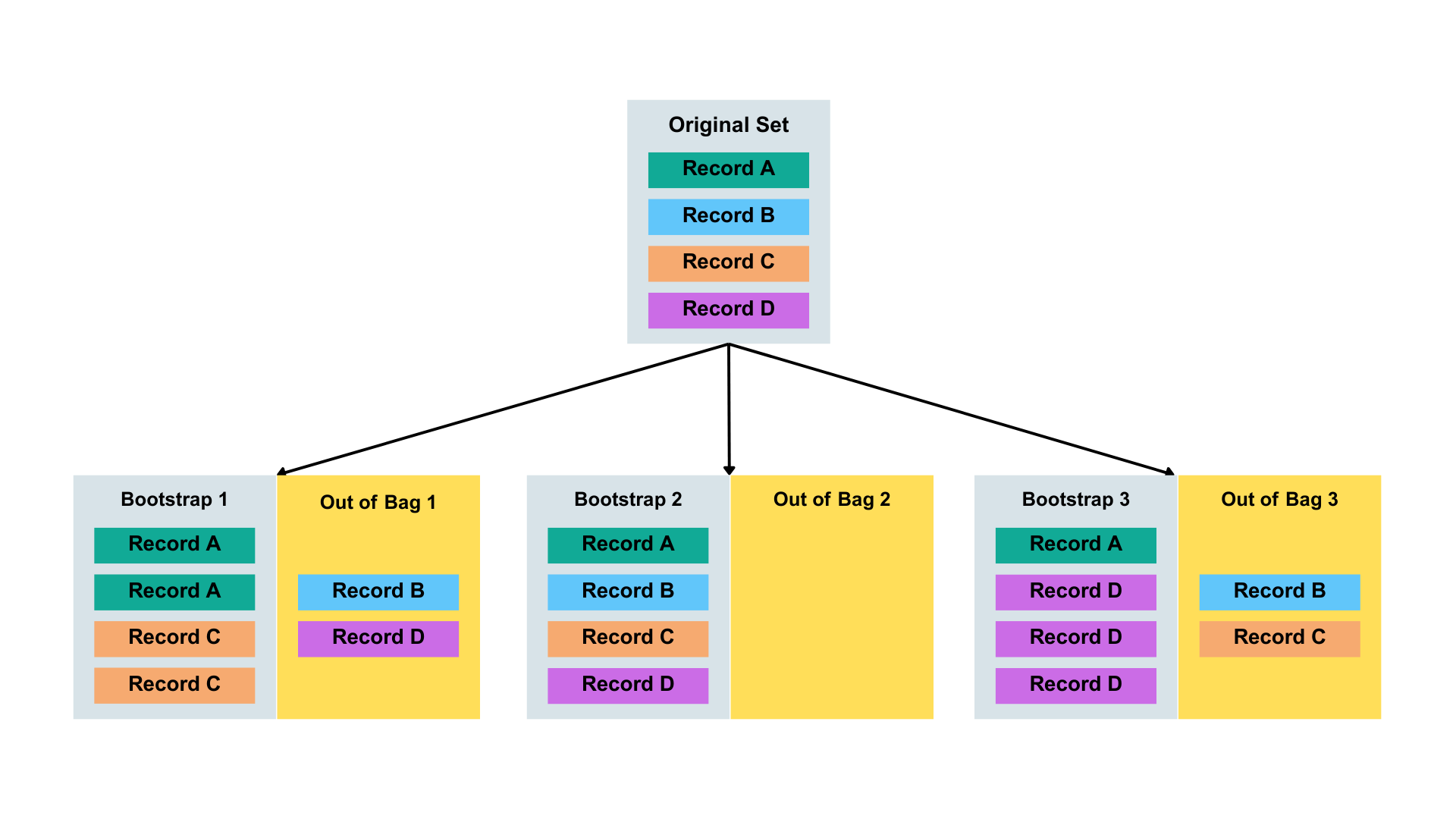
Figure adapted from Smith et al. (2024) and Kwon and Zou (2023).

Random Forest uses these OOB samples as a built-in validation set: For each observation, it’s passed down all the trees where it was OOB. The final OOB prediction is the majority vote (for classification) across those trees. On average, about 1/3 of the data is left our per tree for later in evaluation.

Objectives

Familiarise yourself with the five main steps of running Random Forest for a tree species.
Learn how to adjust this Quarto Markdown notebook to run your own RF-based SDM.
Get accustomed to the style of the EcoCommons Notebooks.
Know the differences between GLM and RF.

Workflow overview

Following a standard protocol for species distribution models proposed by Zurell et al., (2020), a R environment set-up step and five main modelling steps are demonstrated in this notebook:

Step	Main Step	Sub-steps
Set-up	Set-up	S.1 Set up the working directory S.2 Install and load required R packages for this notebook S.3 Download the case study datasets
Step 1	Overview and Conceptualisation Data	1.1 Taxon, location, predictors, scale 1.2 Biodiversity data 1.3 Environmental data 1.4 Combine data
Step 2	Model fitting	2.1 Data splitting 2.2 Model fitting
Step 3	Evaluation	3.1 Model interpretation 3.2 Cross-validation 3.3 Mapping and Interpolation
Step 4	Model comparison	4.1 Number of trees of Random Forest 4.2 Random Forest and GLM

In the near future, this material may form part of comprehensive support materials available to EcoCommons users. If you have any corrections or suggestions to improve the efficiency, please contact the EcoCommons team.

Set-up: R environment and packages

Some housekeeping before we start. This process might take some time as many packages needed to be installed.

S.1 Set the working directory and create a folder for data.

Save the Quarto Markdown file (.QMD) to a folder of your choice, and then set the path to your folder as your working directory.

# Set the workspace to the current working directory
# Uncomment and replace the path below with your own working directory if needed:
# setwd("/Users/zhaoxiang/Documents/tmp/EC_RF_notebook") 

workspace <- getwd()  # Get the current working directory and store it in 'workspace'

# Increase the plot size by adjusting the options for plot dimensions in the notebook output
options(repr.plot.width = 16, repr.plot.height = 8)  # Sets width to 16 and height to 8 for larger plots

S.2 Install and load essential libraries.

Install and load R packages.

# Set CRAN mirror
options(repos = c(CRAN = "https://cran.rstudio.com/"))

# List of packages to check, install if needed, and load
packages <- c("caret", "dplyr", "terra", "sf", "googledrive", "ggplot2", "corrplot", "pROC", "dismo", "spatstat.geom", "patchwork", "biomod2", "leaflet", "car", "gridExtra", "htmltools", "RColorBrewer", "knitr", "kableExtra", "randomForest")

# Function to display a cat message
cat_message <- function(pkg, message_type) {
  if (message_type == "installed") {
    cat(paste0(pkg, " has been installed successfully!\n"))
  } else if (message_type == "loading") {
    cat(paste0(pkg, " is already installed and has been loaded!\n"))
  }
}

# Install missing packages and load them
for (pkg in packages) {
  if (!requireNamespace(pkg, quietly = TRUE)) {
    install.packages(pkg)
    cat_message(pkg, "installed")
  } else {
    cat_message(pkg, "loading")
  }
  library(pkg, character.only = TRUE)
}

caret is already installed and has been loaded!

dplyr is already installed and has been loaded!

terra is already installed and has been loaded!

sf is already installed and has been loaded!

googledrive is already installed and has been loaded!
ggplot2 is already installed and has been loaded!
corrplot is already installed and has been loaded!

pROC is already installed and has been loaded!

dismo is already installed and has been loaded!

spatstat.geom is already installed and has been loaded!

patchwork is already installed and has been loaded!

biomod2 is already installed and has been loaded!

leaflet is already installed and has been loaded!
car is already installed and has been loaded!

gridExtra is already installed and has been loaded!

htmltools is already installed and has been loaded!
RColorBrewer is already installed and has been loaded!
knitr is already installed and has been loaded!

kableExtra is already installed and has been loaded!

randomForest is already installed and has been loaded!

S.3 Download case study datasets

We have prepared the following data and uploaded them to our Google Drive for your use:

Species occurrence data: Shapefile format (.shp)
Environmental variables: Stacked Raster format (.tif)
Study area boundary: Shapefile format (.shp)

# De-authenticate Google Drive to access public files
drive_deauth()

# Define Google Drive file ID and the path for downloading
zip_file_id <- "1wblHSFm1kkZLytNmpEBHnmEajR-bsA35"
datafolder_path <- file.path(workspace)

# Create a local path for the zipped file
zip_file_path <- file.path(datafolder_path, "mountain_ash_centralhighlands_data_RF.zip")

# Function to download a file with progress messages
download_zip_file <- function(file_id, file_path) {
  cat("Downloading zipped file...\n")
  drive_download(as_id(file_id), path = file_path, overwrite = TRUE)
  cat("Downloaded zipped file to:", file_path, "\n")
}

# Create local directory if it doesn't exist
if (!dir.exists(datafolder_path)) {
  dir.create(datafolder_path, recursive = TRUE)
}

# Download the zipped file
cat("Starting to download the zipped file...\n")

Starting to download the zipped file...

download_zip_file(zip_file_id, zip_file_path)

Downloading zipped file...

File downloaded:

• 'mountain_ash_centralhighlands_RF.zip'
  <id: 1wblHSFm1kkZLytNmpEBHnmEajR-bsA35>

Saved locally as:

• '/Users/xiangzhaoqcif/Documents/QCIF_MacBook_Pro/github/notebook-blog/notebooks/EC_RF/mountain_ash_centralhighlands_data_RF.zip'

Downloaded zipped file to: /Users/xiangzhaoqcif/Documents/QCIF_MacBook_Pro/github/notebook-blog/notebooks/EC_RF/mountain_ash_centralhighlands_data_RF.zip

# Unzip the downloaded file
cat("Unzipping the file...\n")

Unzipping the file...

unzip(zip_file_path, exdir = datafolder_path)
cat("Unzipped files to folder:", datafolder_path, "\n")

Unzipped files to folder: /Users/xiangzhaoqcif/Documents/QCIF_MacBook_Pro/github/notebook-blog/notebooks/EC_RF

1 Overview and Conceptualisation

1.1 Taxon, location, and scale

Taxon: Mountain Ash (Eucalyptus regnans)

Mountain Ash,

Photographer: Reiner Richter, ALA

Mountain Ash (Eucalyptus regnans), is a remarkably tall and straight tree native to Victoria and Tasmania. This species thrives in cool, temperate rainforest characterized by high rainfall, deep, well-drained soils, mild temperatures, and high humidity. It is typically found at altitudes ranging from 200 to 1,000 meters above sea level (Burns et al., 2015).

The Mountain Ash faces two main forms of disturbance: bushfires, which are its primary natural disturbance, and logging, which represents the primary human-induced threat to its habitat (Burns et al., 2015; Nevill et al., 2010).

Location: the Central Highlands (study area) in the south part of Victoria

Spatial and temporal scales: small (spatial) and static (temporal)

1.2 Biodiversity data

For this exercise, we have prepared a species occurrence data file in CSV format, which was downloaded from ALA.

central_highlands <- sf::st_read("mountain_ash_centralhighlands_RF/central_highlands.shp")

Reading layer `central_highlands' from data source 
  `/Users/xiangzhaoqcif/Documents/QCIF_MacBook_Pro/github/notebook-blog/notebooks/EC_RF/mountain_ash_centralhighlands_RF/central_highlands.shp' 
  using driver `ESRI Shapefile'
Simple feature collection with 1 feature and 4 fields
Geometry type: POLYGON
Dimension:     XY
Bounding box:  xmin: 144.9398 ymin: -38.20964 xmax: 146.4563 ymax: -36.97746
Geodetic CRS:  GDA94

mountain_ash_centralhighlands <- sf::st_read("mountain_ash_centralhighlands_RF/mountain_ash_centralhighlands.shp")

Reading layer `mountain_ash_centralhighlands' from data source 
  `/Users/xiangzhaoqcif/Documents/QCIF_MacBook_Pro/github/notebook-blog/notebooks/EC_RF/mountain_ash_centralhighlands_RF/mountain_ash_centralhighlands.shp' 
  using driver `ESRI Shapefile'
Simple feature collection with 3933 features and 1 field
Geometry type: POINT
Dimension:     XY
Bounding box:  xmin: 145.0258 ymin: -38.2 xmax: 146.4333 ymax: -37.22625
Geodetic CRS:  GDA94

# Filter the data to include only ABSENT points
mountain_ash_present <- mountain_ash_centralhighlands %>%
  dplyr::filter(occrrnS == "1")

# Filter the data to include only ABSENT points
mountain_ash_absent <- mountain_ash_centralhighlands %>%
  dplyr::filter(occrrnS == "0")

leaflet() %>%
  addProviderTiles(providers$Esri.WorldImagery) %>%
 # Add the Central Highlands layer with a distinct color
  addPolygons(data = central_highlands,
              color = "lightblue",         # Border color of Central Highlands polygon
              weight = 1,            # Border width
              fillColor = "lightblue",  # Fill color of Central Highlands
              fillOpacity = 0.3,     # Transparency for fill
              group = "Central Highlands") %>%
  
    # Add Mountain Ash presence points
  addCircleMarkers(data = mountain_ash_present,
                   color = "#11aa96",
                   radius = 1,
                   weight = 0.5,
                   opacity = 1,
                   fillOpacity = 1,
                   group = "Mountain Ash Presence Records") %>%
  

      # Add Mountain Ash absent points
  addCircleMarkers(data = mountain_ash_absent,
                   color = "#f6aa70",
                   radius = 1,
                   weight = 0.5,
                   opacity = 1,
                   fillOpacity = 1,
                   group = "Mountain Ash Pseudo-absent Records") %>%
  
  setView(lng = 145.7, lat = -37.5, zoom = 7)  %>% # Adjust longitude, latitude, and zoom as needed 
  
    # Add layer controls for easier toggling
  addLayersControl(
    overlayGroups = c("Central Highlands", "Mountain Ash Presence Records", "Mountain Ash Pseudo_absent Records"),
    options = layersControlOptions(collapsed = FALSE)
  ) %>%
  
  # Add a legend for the layers
  addControl(
    html = "
    <div style='background-color: white; padding: 10px; border-radius: 5px;'>
      <strong>Legend</strong><br>
      <i style='background: lightblue; width: 18px; height: 18px; display: inline-block; margin-right: 8px; opacity: 0.7;'></i>
      Central Highlands<br>
      <i style='background: #11aa96; width: 10px; height: 10px; border-radius: 50%; display: inline-block; margin-right: 8px;'></i>
      Mountain Ash Presence Records<br>
      <i style='background: #f6aa70; width: 10px; height: 10px; border-radius: 50%; display: inline-block; margin-right: 8px;'></i>
      Mountain Ash Pseudo-absent Records
    </div>
    ",
    position = "bottomright"
  )

1.3 Environmental Data

💡One core difference between how Random Forest and GLM learn from data is how they react to and deal with multicollinearity in independent variables.

In the GLM notebook, when building SDM with Generalised Linear Model Algorithm, we used correlation matrix and Variance Inflation Factor (VIF) to detect correlation among environmental variables, so that we can select variables that are not highly correlated to avoid issue of multicollinearity. However, such treatment is not necessary for Random Forest. Because while GLM requires linearly independent predictors to ensure reliable inference, Random Forest doesn’t try to separate the independent contribution of each variable. Which means, even if two variables are correlated, the Random Forest model remains stable and robust.

To ensure a valid comparison between RF and GLM, we will use the same set of eight environmental variables as in the GLM notebook.

Environmental Variables Categories	Variables	Data Type	Source
Temperature and Radiation	Bioclim 04: Temperature Seasonality (standard deviation *100) Bioclim 06: Min Temperature of Coldest Month	Continuous	1976-2005, CSIRO via EcoCommons
Humidity	Bioclim 19: Precipitation of Coldest Quarter Bioclim 35: Mean moisture index of coldest quarter	Continuous	1976-2005, CSIRO via EcoCommons
Topography	Digital Elevation Model	Continuous	Geoscience Australia via EcoCommons
Soil	Australian Soil Classification	Categorical	Tern via EcoCommons
Disturbance	Fires Logging	Continuous	Vic DEECA spatial data and resources

# Load the stacked raster layers
env_var_stack <- rast("mountain_ash_centralhighlands_RF/env_stack.tif")

# We want to make sure that soil type raster layer is factor.
env_var_stack[["Soil_Type"]] <- as.factor(env_var_stack[["Soil_Type"]])

# Check if the names are assigned correctly
print(names(env_var_stack))

[1] "Temp_Seasonality"         "Min_Temp_Coldest_Month"  
[3] "Precip_Coldest_Quarter"   "Moisture_Coldest_Quarter"
[5] "Elevation"                "Fires"                   
[7] "Soil_Type"                "Logging"

1.4 Combine species occurrence data and environmental variables

We will create a data frame that combines each presence/absence record of Mountain Ash with data from our 7 environmental variables.

# Extract raster values at species occurrence points
extracted_values  <- terra::extract(env_var_stack, vect(mountain_ash_centralhighlands))

# Drop column of ID
extracted_values <- extracted_values[, !(names(extracted_values) %in% "ID")]

# Combine with species occurrence column
model_data <- data.frame(occurrence = mountain_ash_centralhighlands$occrrnS, extracted_values)

# Remove rows with any NA values in predictors
model_data <- na.omit(model_data)

# we want to make sure the data type of occurrence and soil types are factor.
model_data$occurrence <- as.factor(model_data$occurrence)
model_data$Soil_Type <- as.factor(model_data$Soil_Type)

head(model_data)

  occurrence Temp_Seasonality Min_Temp_Coldest_Month Precip_Coldest_Quarter
1          1         1.424792              2.0631714               13.70784
2          1         1.449565              0.4309082               13.63218
3          1         1.280466              4.2351027               14.27531
4          1         1.390526              1.5544521               13.56016
5          1         1.278574              3.9153066               13.97706
6          1         1.386414              1.6763960               13.54408
  Moisture_Coldest_Quarter Elevation Fires Soil_Type Logging
1                1.0000000  834.7029     0         4       0
2                1.0000000 1058.5144     0         4       3
3                0.9996078  314.3798     0         4       0
4                1.0000000  658.4626     0         7       9
5                1.0000000  544.9786     0         4       0
6                1.0000000  902.7314     0         4       7

2. Model fitting

2.1 Data splitting

For cross-validation purposes, we need to leave out some data as testing dataset. There are many strategies of splitting data for cross-validation, like random, k-fold, and leave-one-out etc. Here we will use the easiest one: random splitting.

# Set seed for reproducibility
set.seed(123)

# Split the data into training (80%) and testing (20%)
train_index <- sample(1:nrow(model_data), size = 0.8 * nrow(model_data))

# Create training and testing datasets
train_data <- model_data[train_index, ]
test_data <- model_data[-train_index, ]

# Check the split
cat("Training Set:", nrow(train_data), "rows\n")

Training Set: 3145 rows

cat("Testing Set:", nrow(test_data), "rows\n")

Testing Set: 787 rows

2.2 Model fitting

2.2.1 Random Forest

We use R package ‘randomForest’ to build our model.

‘ntree’ sets the number of trees to build in the Random Forest. More trees usually have better performance and stability. However, it also means slower computation. Typical values of ‘ntree’ are 500 - 1000 (sometimes 100-200 is enough for fast testing).

‘importance’ is TRUE tells the model to calculate variable importance metrics. This will give you which predictors are most important for explaining the response.

# Fit the model
time_500tree <- system.time({rf_model <- randomForest(
  occurrence ~ .,  # formula: species ~ all other variables
  data = train_data,
  ntree = 500,  # number of trees
  importance = TRUE
)
}) # we can use system.time({}) to know how long does it take to run this model

# Print model summary
print(rf_model)


Call:
 randomForest(formula = occurrence ~ ., data = train_data, ntree = 500,      importance = TRUE) 
               Type of random forest: classification
                     Number of trees: 500
No. of variables tried at each split: 2

        OOB estimate of  error rate: 10.59%
Confusion matrix:
    0    1 class.error
0 984  192  0.16326531
1 141 1828  0.07160995

Number of variables tried at each split (mtry): 2

At each split, 2 predictors were randomly selected to choose the best split — this is the default for classification (√p where p = number of predictors).

Out-of-bag (OOB) error estimate: 10.46%

On average, about 10.5% of samples were misclassified when using only trees that did not see that sample in training (this is an internal cross-validation by Random Forest).

Confusion matrix

Actual class	Predicted 0	Predicted 1	Class error
0 (absence)	989	187	15.9% error → 84.1% correctly predicted
1 (presence)	142	1827	7.2% error → 92.8% correctly predicted

The model is stronger at predicting presence (1) than absence (0). It misclassifies absences more often, which is common when presence points dominate or when background data is noisy.

2.2.2 Generalised Linear Model

# Fit the GLM on the training data
glm_model <- glm(
  occurrence ~ .,
  data = train_data,
  family = binomial(link = "logit")  # Logistic regression
)

3. Model evaluation

3.1 Model interpretation

3.1.1 Random Forest

# Variable importance table
var_imp <- round(as.data.frame(importance(rf_model)), 2) #convert the Random Forest model importance matrix to a dataframe while rounds the numbers to two digits.

kable(var_imp, caption = "Random Forest Variable Importance") %>%
  kable_styling(font_size = 10) #Use knitr::kable() for a clean table

Random Forest Variable Importance
	0	1	MeanDecreaseAccuracy	MeanDecreaseGini
Temp_Seasonality	47.91	46.55	65.75	275.13
Min_Temp_Coldest_Month	50.81	53.53	74.62	230.68
Precip_Coldest_Quarter	35.71	57.49	67.80	325.70
Moisture_Coldest_Quarter	29.10	35.52	47.65	170.35
Elevation	24.52	44.01	55.10	170.43
Fires	1.08	4.48	4.85	0.84
Soil_Type	24.23	43.86	47.68	72.21
Logging	29.57	43.76	49.54	86.78

Mean Decrease Accuracy and Mean Decrease Gini are two commonly used variable importance metrics for Random Forest.

Mean Decrease Accuracy measures how much the model’s prediction accuracy drops when a given variable’s values are randomly permuted.

Mean Decrease Gini measures the total decrease in Gini impurity (a measure of how pure a node is - the greater the decrease in Gini impurity, the more important the variable is considered) caused by splits on a variable, averages over all trees.

✅ Top overall predictors

Min_Temp_Coldest_Month → highest MeanDecreaseAccuracy (71.54) → strongest impact on improving predictive accuracy.
Precip_Coldest_Quarter → second highest (70.40), especially important for predicting presences (1 = 56.94).
Temp_Seasonality → third overall but highest MeanDecreaseGini (269.71) → very important for splitting decisions.

✅ Predictors more important for presences (1) than absences (0)

Precip_Coldest_Quarter (1 = 56.94 vs. 0 = 34.27)
Min_Temp_Coldest_Month (1 = 52.59 vs. 0 = 49.96)
Elevation (1 = 41.35 vs. 0 = 24.37)

3.1.2 Generalised Linear Model

summary(glm_model)


Call:
glm(formula = occurrence ~ ., family = binomial(link = "logit"), 
    data = train_data)

Coefficients:
                           Estimate Std. Error z value Pr(>|z|)    
(Intercept)               1.662e+01  3.074e+01   0.541   0.5887    
Temp_Seasonality         -3.247e+00  1.315e+00  -2.470   0.0135 *  
Min_Temp_Coldest_Month    1.551e+00  9.849e-02  15.750  < 2e-16 ***
Precip_Coldest_Quarter   -4.519e+00  3.233e-01 -13.978  < 2e-16 ***
Moisture_Coldest_Quarter  4.487e+01  2.935e+01   1.529   0.1264    
Elevation                 2.484e-03  4.838e-04   5.133 2.85e-07 ***
Fires                     1.018e-02  9.933e-02   0.103   0.9184    
Soil_Type4                1.949e+00  3.955e-01   4.928 8.31e-07 ***
Soil_Type5               -1.770e-01  4.959e-01  -0.357   0.7211    
Soil_Type7                1.621e+00  4.052e-01   4.002 6.29e-05 ***
Soil_Type8               -1.347e+01  6.038e+02  -0.022   0.9822    
Soil_Type12              -1.336e+01  4.723e+02  -0.028   0.9774    
Soil_Type13              -1.554e+01  1.309e+03  -0.012   0.9905    
Soil_Type14              -1.286e+01  6.500e+02  -0.020   0.9842    
Logging                   1.378e-01  1.514e-02   9.102  < 2e-16 ***
---
Signif. codes:  0 '***' 0.001 '**' 0.01 '*' 0.05 '.' 0.1 ' ' 1

(Dispersion parameter for binomial family taken to be 1)

    Null deviance: 4157.8  on 3144  degrees of freedom
Residual deviance: 2414.8  on 3130  degrees of freedom
AIC: 2444.8

Number of Fisher Scoring iterations: 15

For the interpretation on GLM, please refer to https://ecocommonsaustralia.github.io/notebook-blog/notebooks/EC_GLM/EC_GLM.html

3.2 Cross validation

Now, we use the testing data to evaluate the model performance.

# Predict probabilities and classes
rf_probs <- predict(rf_model, newdata = test_data, type = "prob")[, 2]
rf_preds <- factor(ifelse(rf_probs > 0.5, 1, 0), levels = c(0, 1))

# AUC
rf_roc <- roc(test_data$occurrence, rf_probs, quiet = TRUE)
rf_auc <- auc(rf_roc)
print(rf_auc)

Area under the curve: 0.9317

# Confusion matrix
rf_cm <- confusionMatrix(rf_preds, factor(test_data$occurrence, levels = c(0, 1)), positive = "1")

print(rf_cm)

Confusion Matrix and Statistics

          Reference
Prediction   0   1
         0 218  32
         1  64 473
                                          
               Accuracy : 0.878           
                 95% CI : (0.8531, 0.9001)
    No Information Rate : 0.6417          
    P-Value [Acc > NIR] : < 2.2e-16       
                                          
                  Kappa : 0.7279          
                                          
 Mcnemar's Test P-Value : 0.001557        
                                          
            Sensitivity : 0.9366          
            Specificity : 0.7730          
         Pos Pred Value : 0.8808          
         Neg Pred Value : 0.8720          
             Prevalence : 0.6417          
         Detection Rate : 0.6010          
   Detection Prevalence : 0.6823          
      Balanced Accuracy : 0.8548          
                                          
       'Positive' Class : 1

From above statistics, our model performs very well overall, especially in terms of:

Discriminative power (AUC = 0.932)
High accuracy (0.878) and specificity (0.937)
Good sensitivity — although slightly lower, indicating the model misses some true 0s.
Strong overall agreement (Kappa ~0.73)
Statistical significance across the board

We can also plot the AUC ROC Curve of our model.

# Plot ROC curve
plot(rf_roc, col = "#11aa96", lwd = 1, main = "AUC ROC Curve of the Random Forest model")

# Add AUC as text on the plot
auc_value <- auc(rf_roc)
text(0.6, 0.2, paste("AUC =", round(auc_value, 3)), col = "#11aa96")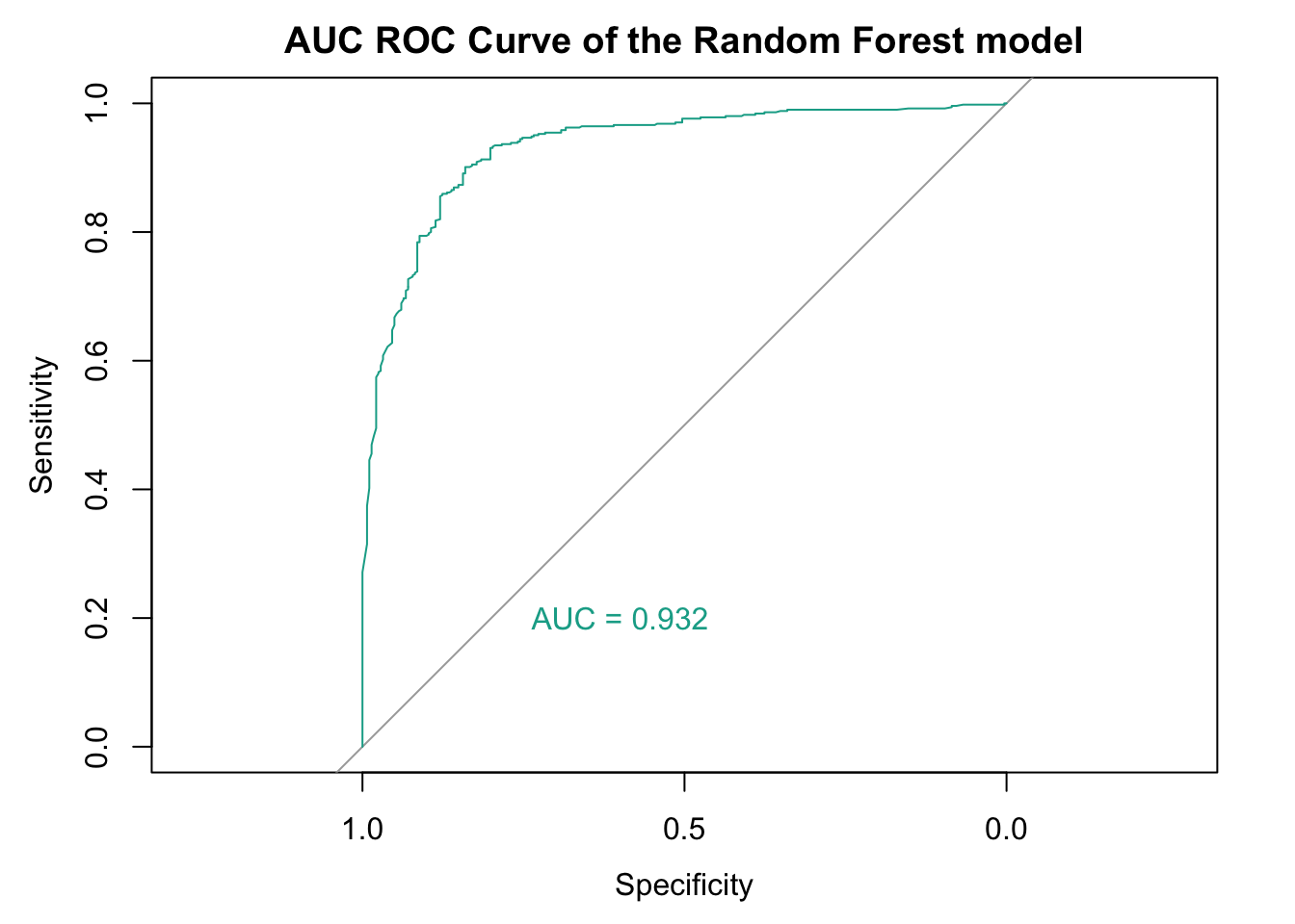

3.3 Mapping and Interpolation

If you remember, we started with these point records of mountain ash

Point data

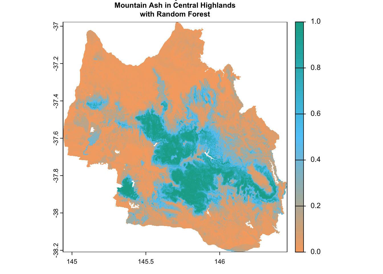
Now, let’s predict a continuous mapping of the distribution of mountain ash in the central highlands.

# Predict the presence probability across the entire raster extent
prediction_rf <- terra::predict(env_var_stack, rf_model, type = "prob", index = 2)

# Define a custom color palette
custom_palette <- colorRampPalette(c("#f6aa70", "#61cafa", "#11aa96"))

# Plot the raster with the custom color palette
plot(
  prediction_rf,
  main = "Predicted Probability of the Presence of\nMountain Ash in Central Highlands\nwith Random Forest",
  col = custom_palette(100),
  cex.main = 0.8
)

We can also use an independent mountain ash data to cross-validate your mapping.

forest_type_vic <- st_read("mountain_ash_centralhighlands_RF/FORTYPE500.shp")

Reading layer `FORTYPE500' from data source 
  `/Users/xiangzhaoqcif/Documents/QCIF_MacBook_Pro/github/notebook-blog/notebooks/EC_RF/mountain_ash_centralhighlands_RF/FORTYPE500.shp' 
  using driver `ESRI Shapefile'
Simple feature collection with 5635 features and 4 fields
Geometry type: POLYGON
Dimension:     XY
Bounding box:  xmin: 140.9631 ymin: -39.23567 xmax: 149.9737 ymax: -33.99701
Geodetic CRS:  GDA94

forest_type_central_highlands <- st_intersection(forest_type_vic, central_highlands)

Warning: attribute variables are assumed to be spatially constant throughout
all geometries

ggplot(data = forest_type_central_highlands) +
  geom_sf(aes(fill = as.factor(X_DESC)), color = NA) +
  scale_fill_manual(
    name = "Forest Type",
    values = c(
      "#D55E00", "#56B4E9", "#009E73", "#F0E442", "#0072B2", 
      "#CC79A7", "#E69F00", "#000000", "#8E44AD", 
      "#3498DB", "#F39C12","#27AE60", "#E74C3C", "#BDC3C7"
    )
  ) +
  labs(title = "Forest Types in the Central Highlands") +
  theme_minimal() +
  theme(
    legend.position = "right",
    legend.text = element_text(size = 8),      # Smaller legend text
    legend.title = element_text(size = 10),   # Smaller legend title
    plot.title = element_text(size = 16, face = "bold"), # Larger plot title
    axis.text = element_text(size = 10),      # Adjust axis text
    axis.title = element_text(size = 12)      # Adjust axis title
  ) +
  coord_sf(expand = FALSE)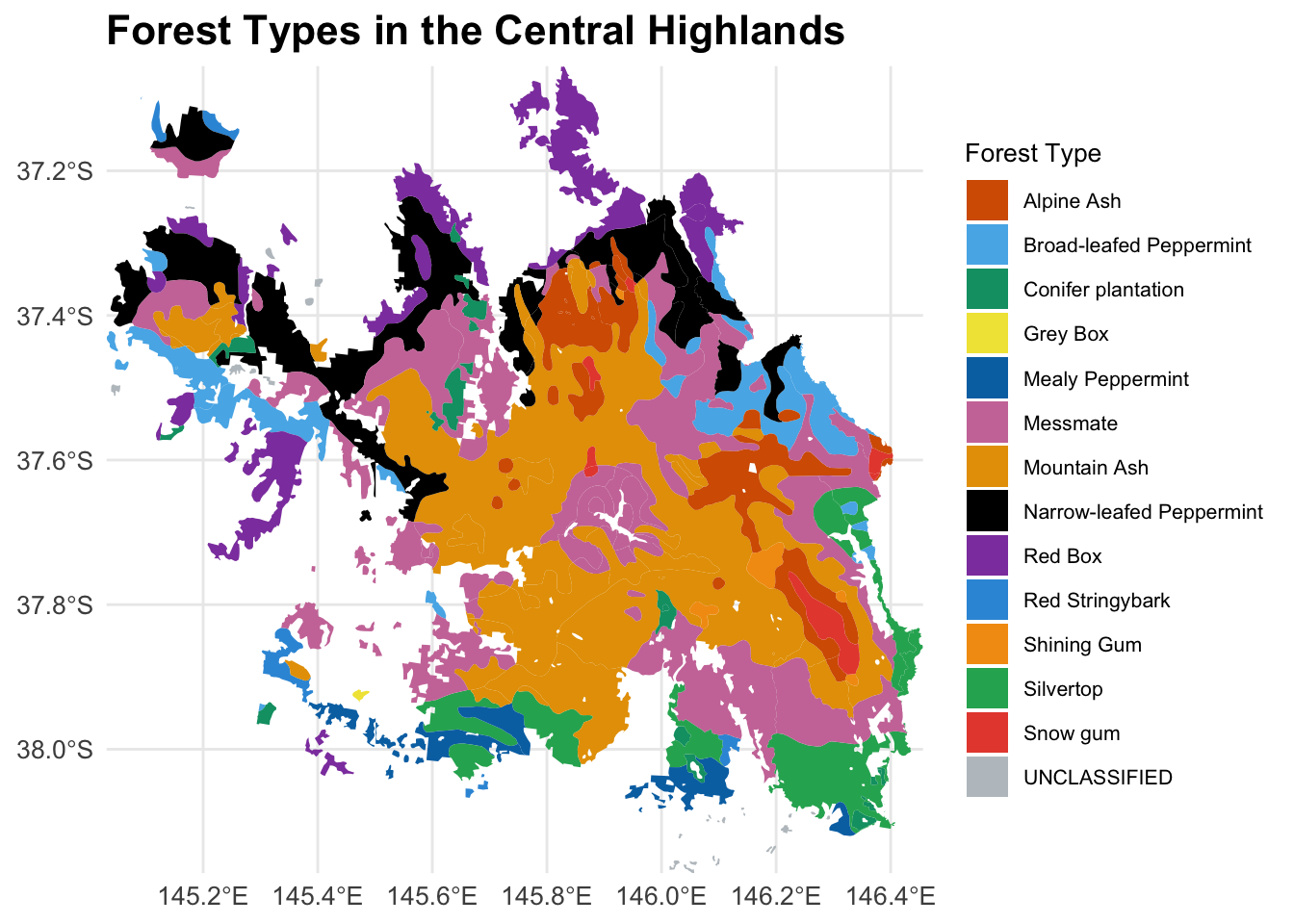

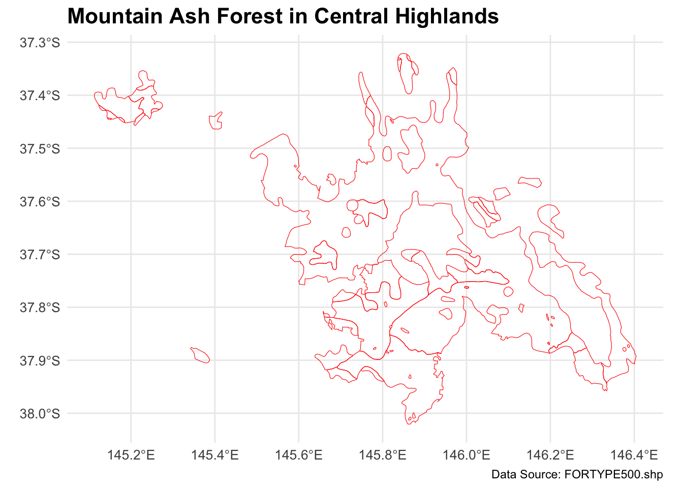
mountain_ash_forest <- forest_type_central_highlands[forest_type_central_highlands$X_DESC == "Mountain Ash", ]

# Plot the filtered shapefile
ggplot(data = mountain_ash_forest) +
  geom_sf(fill = "NA", color = "red", size = 0.1) +  # Blue fill and black border
  labs(
    title = "Mountain Ash Forest in Central Highlands",
    caption = "Data Source: FORTYPE500.shp"
  ) +
  theme_minimal() +
  theme(
    plot.title = element_text(size = 16, face = "bold"),
    axis.text = element_text(size = 10),
    axis.title = element_blank(),
    legend.position = "none"  # No legend needed since this is a single type
  )

custom_palette <- c("#f6aa70", "#61cafa", "#11aa96")


pal <- colorNumeric(
  palette = custom_palette,      # Use custom colors
  domain = values(prediction_rf),
  na.color = "transparent"       # Make NA values transparent
)

# Create the leaflet map
leaflet() %>%
  addProviderTiles(providers$Esri.WorldImagery) %>%
  # Add raster layer
  addRasterImage(prediction_rf, color = pal, opacity = 0.7, project = TRUE) %>%
  # Add shapefile layer
  addPolygons(
    data = mountain_ash_forest,
    color = "red",              # Border color of shapefile polygons
    weight = 1,                  # Border width
    fillColor = "lightblue",     # Fill color of shapefile polygons
    fillOpacity = 0.3            # Transparency for fill
  ) %>%
  # Add legend for raster
  addLegend(
    pal = pal,
    values = values(prediction_rf),
    title = "Probability",
    position = "bottomright"
  )

Warning: sf layer has inconsistent datum (+proj=longlat +ellps=GRS80 +no_defs).
Need '+proj=longlat +datum=WGS84'

4. Model comparison

4.1 Number of trees

As we mentioned in section 2.2.1, a higher number of trees generally leads to greater model accuracy but results in slower computation. Let’s test this.

# Fit the model with 100 trees
time_100tree <- system.time({
rf_model_100tree <- randomForest(
  occurrence ~ .,  # formula: species ~ all other variables
  data = train_data,
  ntree = 100,  # number of trees
  importance = TRUE
)
})

# Fit the model with 1000 trees
time_1000tree <- system.time({
rf_model_1000tree <- randomForest(
  occurrence ~ .,  # formula: species ~ all other variables
  data = train_data,
  ntree = 1000,  # number of trees
  importance = TRUE
)
})

First, let’s compare the computational time of 100, 500, and 1000 trees.

cat("100 trees elapsed time:", time_100tree["elapsed"], "seconds\n")

100 trees elapsed time: 0.3 seconds

cat("500 trees elapsed time:", time_500tree["elapsed"], "seconds\n")

500 trees elapsed time: 2.425 seconds

cat("1000 trees elapsed time:", time_1000tree["elapsed"], "seconds\n")

1000 trees elapsed time: 2.926 seconds

So, more trees do take a longer time to finish.

Let’s see how the OOB error changes among models with different number of trees.

cat("OOB Error (100 trees):", rf_model_100tree$err.rate[nrow(rf_model_100tree$err.rate), "OOB"], "\n")

OOB Error (100 trees): 0.1106518

cat("OOB Error (500 trees):", rf_model$err.rate[nrow(rf_model$err.rate), "OOB"], "\n")

OOB Error (500 trees): 0.1058824

cat("OOB Error (1000 trees):", rf_model_1000tree$err.rate[nrow(rf_model_1000tree$err.rate), "OOB"], "\n")

OOB Error (1000 trees): 0.1065183

The OOB error decreased slightly as the number of trees increased, reaching the lowest point at 500 trees (10.59%). This suggests that 500 trees is likely sufficient for stable and accurate performance, as increasing to 1000 trees yields no further gain but increases computation time.

Now, let’s compare the AUC ROC curves.

# Predict probabilities
pred_100 <- predict(rf_model_100tree, newdata = test_data, type = "prob")[,2]
pred_1000 <- predict(rf_model_1000tree, newdata = test_data, type = "prob")[,2]

# Calculate ROC curves
roc_100 <- roc(test_data$occurrence, pred_100, quiet = TRUE)
roc_1000 <- roc(test_data$occurrence, pred_1000, quiet = TRUE)

# Plot ROC curves
plot(roc_100, col = "lightblue", lwd = 2, main = "ROC Curves Comparison", legacy.axes = TRUE)
plot(rf_roc, col = "#11aa96", lwd = 2, add = TRUE)
plot(roc_1000, col = "#f6aa70", lwd = 2, add = TRUE)
abline(a = 0, b = 1, lty = 2, col = "gray")  # diagonal reference line

# Add AUC legend
legend("bottomright",
       legend = c(
         paste("100 trees (AUC =", round(auc(roc_100), 3), ")"),
         paste("500 trees (AUC =", round(auc(rf_roc), 3), ")"),
         paste("1000 trees (AUC =", round(auc(roc_1000), 3), ")")
       ),
       col = c("lightblue", "#11aa96", "#f6aa70"),
       lwd = 2,
       cex = 0.5,         # Shrinks text size
       inset = 0.02      # Pushes legend slightly inside the plot
)

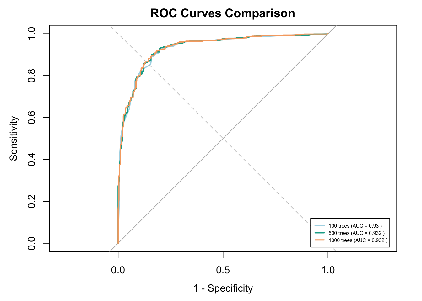
In this case, increasing the number of trees doesn’t significantly improve the AUC of the model.

4.2 Random Forest and GLM

Now, let’s compare the Random Forest model and GLM model.

First, we need to compute the cross validation for GLM like we did for RF.

# Predict probabilities and classes
glm_probs <- predict(glm_model, newdata = test_data, type = "response")
glm_preds <- factor(ifelse(glm_probs > 0.5, 1, 0), levels = c(0, 1))

# AUC
glm_roc <- roc(test_data$occurrence, glm_probs, quiet = TRUE)
glm_auc <- auc(glm_roc)

# Confusion matrix
glm_cm <- confusionMatrix(glm_preds, factor(test_data$occurrence, levels = c(0, 1)), positive = "1")

4.2.1 AUC-ROC curve

Let’s compare the AUC-ROC curve of each algorithm.

plot(rf_roc, col = "#11aa96", lwd = 2, main = "RF vs. GLM ROC Curve")
plot(glm_roc, col = "purple", lwd = 2, add = TRUE)
abline(a = 0, b = 1, lty = 2, col = "gray")

legend("bottomright",
       legend = c(paste("RF (AUC =", round(auc(rf_roc), 3), ")"),
                  paste("GLM (AUC =", round(auc(glm_roc), 3), ")")),
       col = c("#11aa96", "purple"),
       lwd = 2,
       cex = 0.8,
       bty = "n")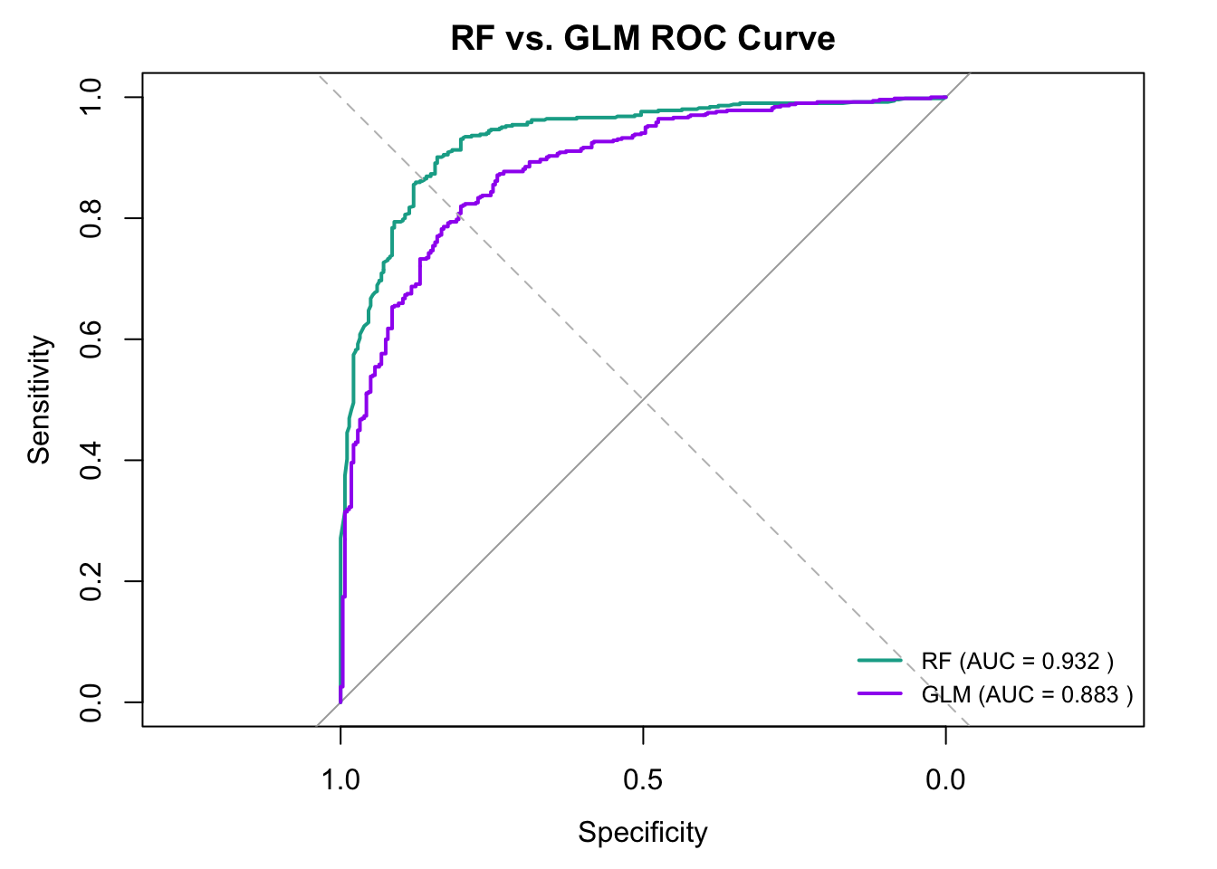

The ROC curve shows that the Random Forest model outperforms the GLM model in classifying the binary outcome. With an AUC of 0.932 vs 0.883, RF achieves higher sensitivity and specificity across a range of thresholds, making it a more reliable model for this dataset.

4.2.2 Importance of variables

We can also see how two algorithms rank the importance of variables.

# Calculate Random Forest importance
rf_importance <- importance(rf_model)
rf_importance_df <- as.data.frame(rf_importance)
rf_importance_df$Variable <- rownames(rf_importance_df)

# Sort RF variables by importance
rf_sorted <- rf_importance_df[order(-rf_importance_df$MeanDecreaseAccuracy), "Variable"]

# Calculate GLM importance (absolute coefficients)
glm_summary <- summary(glm_model)
glm_coeffs <- glm_summary$coefficients
glm_coeffs <- glm_coeffs[-1, , drop = FALSE]

glm_importance_df <- data.frame(
  Variable = rownames(glm_coeffs),
  Coefficient = glm_coeffs[, "Estimate"],
  Abs_Coefficient = abs(glm_coeffs[, "Estimate"])
)

# Sort GLM variables by absolute coefficient
glm_sorted <- glm_importance_df[order(-glm_importance_df$Abs_Coefficient), "Variable"]

# Get maximum length
max_len <- max(length(rf_sorted), length(glm_sorted))

# Pad shorter list with NA
rf_sorted <- c(rf_sorted, rep(NA, max_len - length(rf_sorted)))
glm_sorted <- c(glm_sorted, rep(NA, max_len - length(glm_sorted)))

# Create comparison table
comparison_table <- data.frame(
  Rank = 1:max_len,
  Random_Forest = rf_sorted,
  GLM = glm_sorted
)

kable(comparison_table, caption = "All Variables: Random Forest vs GLM (sorted by importance)") %>% kable_styling(font_size = 10) #Use knitr::kable() for a clean table

All Variables: Random Forest vs GLM (sorted by importance)
Rank	Random_Forest	GLM
1	Min_Temp_Coldest_Month	Moisture_Coldest_Quarter
2	Precip_Coldest_Quarter	Soil_Type13
3	Temp_Seasonality	Soil_Type8
4	Elevation	Soil_Type12
5	Logging	Soil_Type14
6	Soil_Type	Precip_Coldest_Quarter
7	Moisture_Coldest_Quarter	Temp_Seasonality
8	Fires	Soil_Type4
9	NA	Soil_Type7
10	NA	Min_Temp_Coldest_Month
11	NA	Soil_Type5
12	NA	Logging
13	NA	Fires
14	NA	Elevation

As you can see in above table, these two algorithms rank the importance of variables differently.

Random Forest (RF)

RF ranks climatic variables like Min_Temp_Coldest_Month, Precip_Coldest_Quarter, and Temp_Seasonality as most important.
It uses numeric, continuous variables effectively for splitting decision trees.
Categorical variables like Soil_Type and Logging appear, but with less influence.

GLM

GLM relies heavily on individual levels of categorical variables (e.g., Soil_Type13, Soil_Type8, etc.).
This is expected because GLMs break down categorical variables into separate coefficients per level.
Some continuous variables like Moisture_Coldest_Quarter and Precip_Coldest_Quarter also contribute, but generally less prominently.

💡 Another difference between Random Forest and GLM is how they deal with individual levels of categorical variables. GLM is a parametric, equation-based model. It needs numeric inputs, so it transforms categorical variables into dummy (indicator) variables. The model estimates separate regression coefficients for each level (relative to the reference). That’s why you can see Soil_Type13, Soil_Type8, etc listed in the above table.

RF is a non-parametric, tree-based model. It doesn’t need dummy variables — it can handle categorical variables natively (if they are encoded as factors in R). However, variable importance is reported for the entire variable, not per level. That’s why you can only find Soil_Type in the above table instead of each levels of soil type.

4.2.3 Performance statistics

Now, let’s compare the model statistics of two algorithms.

# Extract stats
extract_stats <- function(cm, auc_val) {
  c(
    Accuracy = cm$overall["Accuracy"],
    Kappa = cm$overall["Kappa"],
    Sensitivity = cm$byClass["Sensitivity"],
    Specificity = cm$byClass["Specificity"],
    Precision = cm$byClass["Pos Pred Value"],
    F1 = cm$byClass["F1"],
    AUC = auc_val
  )
}

rf_stats <- extract_stats(rf_cm, rf_auc)
glm_stats <- extract_stats(glm_cm, glm_auc)

# Combine into a comparison table
comparison_table <- data.frame(
  Metric = names(rf_stats),
  Random_Forest = round(as.numeric(rf_stats), 4),
  GLM = round(as.numeric(glm_stats), 4)
)

# Print result
print(comparison_table)

                    Metric Random_Forest    GLM
1        Accuracy.Accuracy        0.8780 0.8145
2              Kappa.Kappa        0.7279 0.5869
3  Sensitivity.Sensitivity        0.9366 0.8851
4  Specificity.Specificity        0.7730 0.6879
5 Precision.Pos Pred Value        0.8808 0.8355
6                    F1.F1        0.9079 0.8596
7                      AUC        0.9317 0.8829

The Random Forest model outperforms the GLM model across all major performance metrics. It has higher accuracy, better class separation (AUC), stronger precision and recall balance (F1), and greater agreement with actual outcomes (Kappa). This suggests RF is a more robust classifier on this dataset, both in predictive power and error balance.

4.2.4 Prediction map comparison

# Predict the presence probability using the GLM model over the raster stack
prediction_glm <- terra::predict(env_var_stack, glm_model, type = "response")

# Calculate difference raster
prediction_diff <- prediction_rf - prediction_glm

# Define custom color palette
custom_palette <- colorRampPalette(c("#f6aa70", "#61cafa", "#11aa96"))
diff_palette <- colorRampPalette(c("red", "white", "blue"))

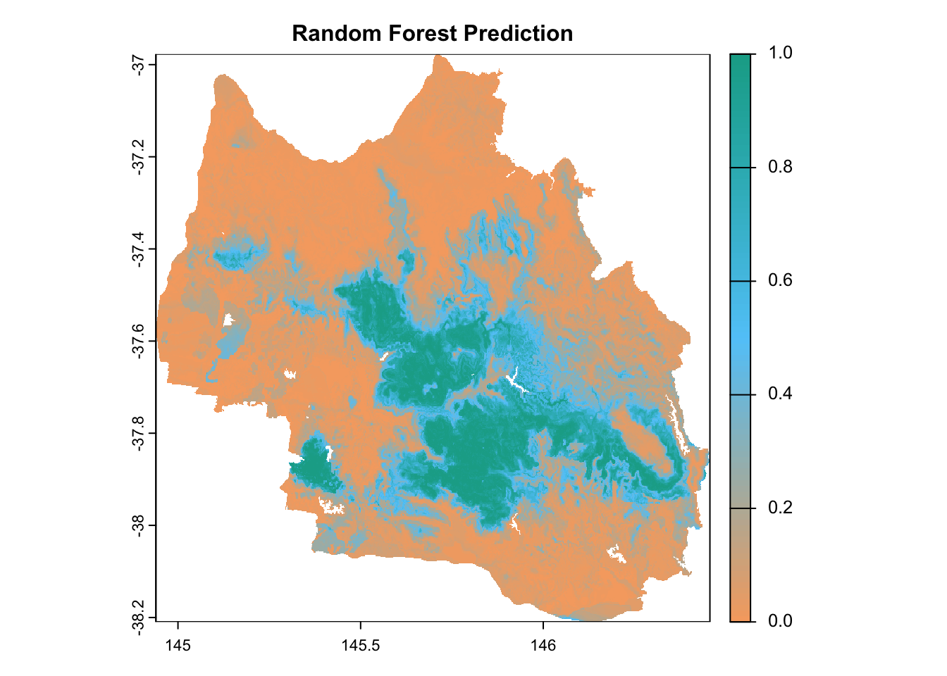
# 1. Random Forest prediction
plot(
  prediction_rf,
  main = "Random Forest Prediction",
  col = custom_palette(100),
  cex.main = 1
)

# 2. GLM prediction
plot(
  prediction_glm,
  main = "GLM Prediction",
  col = custom_palette(100),
  cex.main = 1
)

# 3. Difference map
plot(
  prediction_diff,
  main = "Difference (RF - GLM)",
  col = diff_palette(100),
  cex.main = 1
)

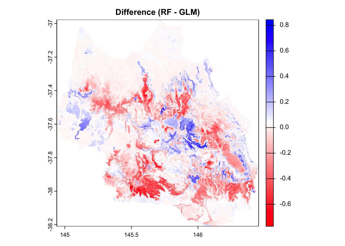
Interpretation of Color Scale

Red areas → GLM predicts higher probabilities than Random Forest (RF).
Blue areas → RF predicts higher probabilities than GLM.
White areas → Both models predict similar probabilities (difference near 0).

Spatial Insight

There is a clear spatial structure in model disagreement. Some regions are consistently blue or red, suggesting systematic differences in how each model interprets environmental features.

What to do next

Investigate which environmental variables contribute most to these differences.
Consider plotting variable importance for both models to understand their decision mechanisms.
Optionally, explore these differences using residual maps, partial dependence plots, or a stacked ensemble model.

4.2.5 When to use what

⚠️ Here comes the question: if Random Forest model is always better, then when should we use GLM?

A short answer to this question is:

Use GLM when you need statistical interpretation and inference; use Random Forest when you prioritize prediction accuracy and can tolerate less interpretability.

Use GLM when:

Interpretability is important

GLM gives explicit coefficients for each predictor. Refering to 3.1.2 Generalised Linear Model, you get p-values, confidence intervals, and direction (positive/negative effect), which RF does not provide.

You need statistical inference

GLM gives you significance tests, effect size, and model diagnostics. However, RF is more like a black box - you don’t get p-values or causal interpretation.

Your data is small

RF can overfit or behave unstably on small datasets. GLM is simpler, more stable, and works well with limited data.

Your variables are mostly linear and well-understood

If relationships are linear and the model is well specified, GLM can be nearly as accurate — and much easier to explain.

Use RF when:

You care more about prediction than interpretation

Data is large, complex, non-linear, or has interactions

You’re doing machine learning, not inference

You want to automate decisions, not explain them

5. Summary

In this notebook, we explored how the Random Forest algorithm works, introducing key concepts such as decision tree, bootstrap sampling and the out-of-bag (OOB) validation method.

We then talked through the complete process of building a Random Forest model and interpreting its performance using metrix like Mean Decrease Accuracy and Mean Decrease Gini.

Finally, we compared Random Forest and Generalised Linear Model, highlighting key differences between in how each algorithm handles variable importance, multicollinearity and model interpretation:

💡GLM is sensitive to multicollinearity and requires the removal of highly correlated predictors to ensure reliable inference, typically using tools like correlation matrices and VIF. In contrast, Random Forest is robust to multicollinearity because it doesn’t rely on estimating independent contributions of each variable, allowing correlated variables to coexist without degrading model performance.

💡GLM transforms categorical variables into dummy variables and estimates separate coefficients for each level, allowing detailed interpretation of individual categories. In contrast, Random Forest handles categorical variables natively and reports importance at the whole-variable level, not for individual levels.

We also discussed the advantages and disadvantages of using these two algorithms:

Use GLM when interpretability, statistical inference, or understanding variable effects is important—especially with small or well-structured data. It provides coefficients, p-values, and confidence intervals, making it ideal for transparent analysis.

Use Random Forest when your goal is prediction over explanation, particularly with large, complex, or non-linear data. While less interpretable, it handles interactions and multicollinearity robustly and often achieves higher predictive accuracy.

References

Breiman, L. (2001), Random Forests, Machine Learning 45(1), 5-32.

Burns, E. L., Lindenmayer, D. B., Stein, J., Blanchard, W., McBurney, L., Blair, D., & Banks, S. C. (2015). Ecosystem assessment of mountain ash forest in the C entral H ighlands of V ictoria, south‐eastern A ustralia. Austral Ecology, 40(4), 386-399.

Kwon, Y., & Zou, J. (2023, July). Data-oob: Out-of-bag estimate as a simple and efficient data value. In International conference on machine learning (pp. 18135-18152). PMLR.

Nevill, P. G., Bossinger, G., & Ades, P. K. (2010). Phylogeography of the world’s tallest angiosperm, Eucalyptus regnans: evidence for multiple isolated Quaternary refugia. Journal of Biogeography, 37(1), 179-192.

Smith, H. L., Biggs, P. J., French, N. P., Smith, A. N., & Marshall, J. C. (2024). Out of (the) bag—encoding categorical predictors impacts out-of-bag samples. PeerJ Computer Science, 10, e2445.

von Takach Dukai, B. (2019). The genetic and demographic impacts of contemporary disturbance regimes in mountain ash forests.

Zurell, D., Franklin, J., König, C., Bouchet, P. J., Dormann, C. F., Elith, J., Fandos, G., Feng, X., Guillera‐Arroita, G., & Guisan, A. (2020). A standard protocol for reporting species distribution models. Ecography, 43(9), 1261-1277.

Logging History (1930-07-01 - 2022-06-30), Data VIC, 2024, https://discover.data.vic.gov.au/dataset/logging-history-overlay-of-most-recent-harvesting-activities

Fire History (2011-2021), Data VIC, 2024, https://www.agriculture.gov.au/abares/forestsaustralia/forest-data-maps-and-tools/spatial-data/forest-fire#fires-in-australias-forests-201116-2018

Harwood, Tom (2019): 9s climatology for continental Australia 1976-2005: BIOCLIM variable suite. v1. CSIRO. Data Collection. https://doi.org/10.25919/5dce30cad79a8

3 second SRTM Derived Digital Elevation Model (DEM) Version 1.0, Geoscience Australia, 2018, https://dev.ecat.ga.gov.au/geonetwork/srv/api/records/a05f7892-ef04-7506-e044-00144fdd4fa6

Searle, R. (2021): Australian Soil Classification Map. Version 1. Terrestrial Ecosystem Research Network. (Dataset). https://doi.org/10.25901/edyr-wg85