Copyright statement: This script is the product of the EcoCommons platform. Please refer to the EcoCommons website for more details: https://www.ecocommons.org.au/
Date: March 2026
Script and Data Information
This notebook provides a simple, reproducible example of converting a GeoTIFF raster (.tif) into a NetCDF (.nc) using the terra package in R. It is intended as a lightweight template that can be adapted to other raster-based spatial datasets and workflows requiring NetCDF outputs.
Other file formats of this notebook
Notebook
Files
Open in Colab / ARDC Jupyter
DOI
GeoTIFF to NetCDF
Introduction
Raster datasets are a common way to represent spatial information in environmental and ecological modelling. Formats such as GeoTIFF (.tif) store spatial data as a grid of cells, where each cell contains a value representing a variable such as temperature, precipitation, or population density. Another widely used raster format is NetCDF (.nc), which is designed to store multidimensional scientific data and is commonly used for climate, oceanographic, and atmospheric datasets.
In many workflows, it is necessary to convert raster data between formats to ensure compatibility with different software tools, data platforms, or modelling frameworks. For example, GeoTIFF files are widely supported by GIS software, while NetCDF is often used for storing large environmental datasets that include multiple variables or time steps.
Although format conversion is often considered a routine technical step, preserving spatial metadata during this process is essential. Changes to key properties such as the coordinate reference system (CRS), spatial extent, or grid resolution can introduce subtle spatial misalignment that may not be immediately visible but can affect downstream analyses and modelling results.
This notebook demonstrates a structured and transparent workflow for converting a GeoTIFF raster (.tif) to a NetCDF file (.nc) while explicitly verifying that important spatial properties—including CRS, extent, and resolution—are preserved during the conversion process.
Key Concepts
K.1 Raster data structure
Raster datasets represent spatial information as a regular grid of cells, where each cell contains a value corresponding to a measured or modelled variable. Raster formats are well suited to continuous surfaces such as climate variables, elevation, or habitat suitability layers.
K.2 NetCDF data formats
NetCDF (Network Common Data Form) is a widely used format for storing multidimensional scientific data. Environmental datasets such as temperature, humidity, pressure, wind speed, and population density are often distributed in NetCDF format because it supports multiple variables and dimensions (e.g. time, latitude, longitude) within a single file.
K.3 Converting raster formats
Converting raster data between formats (e.g. GeoTIFF → NetCDF) is a common preprocessing step that enables compatibility with different software tools, data platforms, and modelling workflows. While GeoTIFF files are widely used in GIS applications, NetCDF is commonly used for storing large environmental datasets that include multiple variables or temporal dimensions. A robust conversion workflow should ensure that key spatial properties—including the coordinate reference system (CRS), spatial extent, and grid resolution—are preserved.
Notebook Objectives
Demonstrate how to read a GeoTIFF (.tif) raster file into R as a SpatRaster using the terra package.
Perform a basic visual check (plot) to confirm that the raster has been loaded correctly.
Convert the raster to a NetCDF (.nc) format and save the output while preserving the original file naming and providing a transparent output location.
Verify that key spatial metadata (CRS, extent, and geometry validity) are preserved during the conversion process.
Workflow Overview
This notebook follows a simple, linear workflow to convert a GeoTIFF raster to a NetCDF (.nc) format via the following steps:
Step 1: Set up the R environment and load the required packages (terra, sf and googledrive).
Step 2: Define and validate the file path to the input GeoTIFF (.tif) raster.
Step 3: Read the raster into R as a SpatRaster object and confirm that a valid CRS is defined.
Step 4: Perform a visual check by plotting the raster to confirm it was read correctly.
Step 5: Export the raster to NetCDF (.nc) format, preserving the original file name and providing a transparent output location.
Step 6: Validate that CRS, spatial extent, and geometry integrity are preserved after conversion.
In the near future, this material may form part of comprehensive support materials available to EcoCommons users. If you have any corrections or suggestions to improve the efficiency, please contact the EcoCommons team.
Step 1. Install and load required packages
Install and load R packages that are not already present in the working environment. For this notebook, the terra, sf and googledrive packages are required for converting a GeoTIFF (.tif) raster to a NetCDF (.nc) and for verifying spatial metadata during the workflow.
# Install and load required packages (if not already installed)required_packages <-c("terra","googledrive","sf","ncdf4")for (pkg in required_packages) {# Install if missingif (!pkg %in%installed.packages()[, "Package"]) {install.packages(pkg)cat("Package installed successfully:", pkg, "\n") }# Load quietlysuppressPackageStartupMessages(library(pkg, character.only =TRUE) )cat("Package loaded successfully:", pkg, "\n")}
Package loaded successfully: terra
Package loaded successfully: googledrive
Package loaded successfully: sf
Package loaded successfully: ncdf4
Step 2. Define the path to the input GeoTIFF raster file
We have provided an example GeoTIFF (.tif) for this notebook via OPTION 2 – Google Drive. If you would like to use your own GeoTIFF, choose OPTION 1, commenting out this line:
tif_file <- NULL
and uncomment this line with your updated path:
tif_file <- "/path_to_your_file
The example GeoTIFF is a binary prediction of suitable habitat for a modelled bird species. Converting a raster (.tif) to NetCDF (.nc) is generally recommended for categorical rasters or rasters that have been reclassified into a small number of categories, rather than for continuous prediction rasters (a common output of species distribution modelling).
Note: The input GeoTIFF raster must have a valid Coordinate Reference System (CRS) defined. If the file does not contain CRS information, the conversion will stop.
# OPTION 1: User-defined local GeoTIFF filetif_file <-NULL#tif_file <- "/path_to_your_file"# OPTION 2: Download example GeoTIFF if no local fileif (is.null(tif_file)) {drive_deauth() workspace <-getwd() datafolder_path <-file.path(workspace, "data")if (!dir.exists(datafolder_path)) {dir.create(datafolder_path, recursive =TRUE) } tif_file_id <-"18HWnL4pgqy08zyik0y_XpGYQwl-qOk05"# Get file metadata (to retrieve original name) file_info <-drive_get(as_id(tif_file_id))# Build full local path using original filename tif_file <-file.path(datafolder_path, file_info$name)# Download to that exact file pathdrive_download(as_id(tif_file_id),path = tif_file,overwrite =TRUE )}
# Final safety checkif (!file.exists(tif_file)) {stop("Input GeoTIFF file not found.")}# Extract base file name (used downstream)base_name <- tools::file_path_sans_ext(basename(tif_file))
Step 3. Read GeoTIFF raster into R
The rast() function reads the GeoTIFF (.tif) file into R as a SpatRaster object.
# Read the GeoTIFF into R as a SpatRaster objectinput_raster <-rast(tif_file)cat("CRS of input raster:\n")
CRS of input raster:
print(crs(input_raster))
[1] "GEOGCRS[\"WGS 84\",\n ENSEMBLE[\"World Geodetic System 1984 ensemble\",\n MEMBER[\"World Geodetic System 1984 (Transit)\"],\n MEMBER[\"World Geodetic System 1984 (G730)\"],\n MEMBER[\"World Geodetic System 1984 (G873)\"],\n MEMBER[\"World Geodetic System 1984 (G1150)\"],\n MEMBER[\"World Geodetic System 1984 (G1674)\"],\n MEMBER[\"World Geodetic System 1984 (G1762)\"],\n MEMBER[\"World Geodetic System 1984 (G2139)\"],\n MEMBER[\"World Geodetic System 1984 (G2296)\"],\n ELLIPSOID[\"WGS 84\",6378137,298.257223563,\n LENGTHUNIT[\"metre\",1]],\n ENSEMBLEACCURACY[2.0]],\n PRIMEM[\"Greenwich\",0,\n ANGLEUNIT[\"degree\",0.0174532925199433]],\n CS[ellipsoidal,2],\n AXIS[\"geodetic latitude (Lat)\",north,\n ORDER[1],\n ANGLEUNIT[\"degree\",0.0174532925199433]],\n AXIS[\"geodetic longitude (Lon)\",east,\n ORDER[2],\n ANGLEUNIT[\"degree\",0.0174532925199433]],\n USAGE[\n SCOPE[\"Horizontal component of 3D system.\"],\n AREA[\"World.\"],\n BBOX[-90,-180,90,180]],\n ID[\"EPSG\",4326]]"
# Stop if CRS is missingif (is.na(crs(input_raster)) ||crs(input_raster) =="") {stop("❌ Input GeoTIFF raster has NO CRS defined.\n","Please ensure the file has a valid CRS before proceeding." )}
Step 4. Plot raster
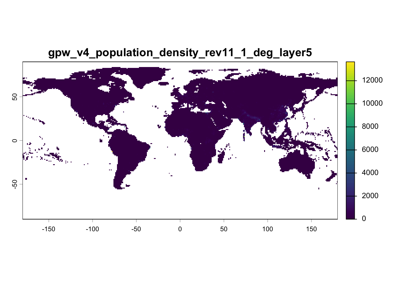
Plot the raster to confirm that it has been read correctly into R before proceeding with conversion. At this stage, the raster exists only as an in-memory SpatRaster object and has not yet been converted or written to disk.
plot(input_raster, main = base_name)
Step 5. Convert raster to NectCDF and save
Now convert the raster to a NetCDF and also save and plot the converted file. By default, the output is written to the same directory as the input raster (.tif) file. We also produce a plot to visually check the GeoTIFF (.tif) to NetCDF (.nc) conversion.
# Define output directory (same as input raster)out_dir <-dirname(tif_file)# Build output file nameout_file <-file.path(out_dir, paste0(base_name, ".nc"))# Write raster to NetCDFterra::writeCDF( input_raster,filename = out_file,overwrite =TRUE)cat("NetCDF written to:\n", out_file, "\n")
NetCDF written to:
 /Users/xiangzhaoqcif/dev/notebook-blog/notebooks/raster_format/data/gpw_v4_population_density_rev11_1_deg_layer5.nc
Step 6. Verify spatial metadata after writing NetCDF
Reload the NetCDF and confirm that CRS, extent, and geometry integrity have been preserved.
# Reload written NetCDFwritten_raster <- terra::rast(out_file)# ---- CRS check ----# Extract CRS info for input rasterinput_crs_info <- terra::crs(input_raster, describe =TRUE)input_crs_name <- input_crs_info$nameinput_epsg <- input_crs_info$code# Extract CRS info for output rasteroutput_crs_info <- terra::crs(written_raster, describe =TRUE)output_crs_name <- output_crs_info$nameoutput_epsg <- output_crs_info$codecat("\nInput CRS name:", input_crs_name, "\n")
if (!isTRUE(all.equal( terra::res(input_raster), terra::res(written_raster)))) {stop("❌ Resolution mismatch detected after writing NetCDF.")}cat("\n✅ All spatial metadata successfully preserved during conversion.\n")
✅ All spatial metadata successfully preserved during conversion.
Summary
This notebook demonstrated a simple, reproducible workflow for converting a GeoTIFF (.tif) raster to NetCDF (.nc) format using the terra package in R. The workflow also verified that key spatial metadata—including the coordinate reference system (CRS), spatial extent, and grid resolution—were preserved during the conversion process.
A companion notebook (link below) demonstrates the reverse workflow, converting NetCDF (.nc) data to GeoTIFF (.tif) format.
Center For International Earth Science Information Network-CIESIN-Columbia University. (2017). Gridded Population of the World, Version 4 (GPWv4): Population Density, Revision 11 (Version 4.11) [Data set]. Palisades, NY: NASA Socioeconomic Data and Applications Center (SEDAC). https://doi.org/10.7927/H49C6VHW Date Accessed: 2026-03-08
How to cite this Notebook
Zhao, X. Y., & Newis, R. (2026). Converting GeoTIFF (.tif) to NetCDF (.nc) Format (Version 1.0) [Computational notebook]. Zenodo. https://doi.org/10.5281/zenodo.19548851
footer
EcoCommons received investment (https://doi.org/10.3565/chbq-mr75) from the Australian Research Data Commons (ARDC). The ARDC is enabled by the National Collaborative Research Infrastructure Strategy (NCRIS).
Our Partner
How to Cite EcoCommons
If you use EcoCommons in your research, please cite the platform as follows: