Getting Shorebird Data in Australia Using Global Biodiversity Data Portals via spocc R Package

Author details: Abhimanyu Raj Singh

Editor details: Xiang Zhao

Contact details: support@ecocommons.org.au

Copyright statement: This script is the product of the EcoCommons platform. Please refer to the EcoCommons website for more details: https://www.ecocommons.org.au/

Date: June 2025

🚀 Before You Start

• Ensure you have a stable internet connection, as species data is fetched live from biodiversity data portals using spocc R package.
• This notebook may take a few minutes when downloading large datasets or installing missing packages.
• Recommended to run in RStudio or Posit Workbench/VS Code with Quarto installed for best experience.

Introduction

This notebook was developed by the EcoCommons team to support researchers and conservationists in gathering shorebird distribution data using open data sources. It demonstrates how to query, clean, visualise, and save species occurrence data using the spocc R package [@spocc] (Chamberlain et al., 2024), in R.

spocc – Species Occurrence Data Aggregator

The spocc package provides a unified interface to search and retrieve species occurrence data from multiple biodiversity data sources into a single workflow. It streamlines data acquisition for ecological modelling and biodiversity analysis by handling different APIs in one place.

We will introduce three of the most popular and largest biodiversity data portals that provide users with the ability to download their data via their platforms or several R packages.

GBIF – Global Biodiversity Information Facility An international network providing open access to data on all types of life on Earth, supporting global biodiversity research and conservation.

iNaturalist – Citizen Science Biodiversity Network A community-driven platform where people record and share species observations, contributing to real-time biodiversity mapping across the globe.

OBIS – Ocean Biodiversity Information System The world’s largest marine biodiversity database, offering access to global data on the distribution of marine life for science, policy, and conservation.

We focus on three key migratory shorebird species, each represented by a distinct colour for clarity in visualisations:

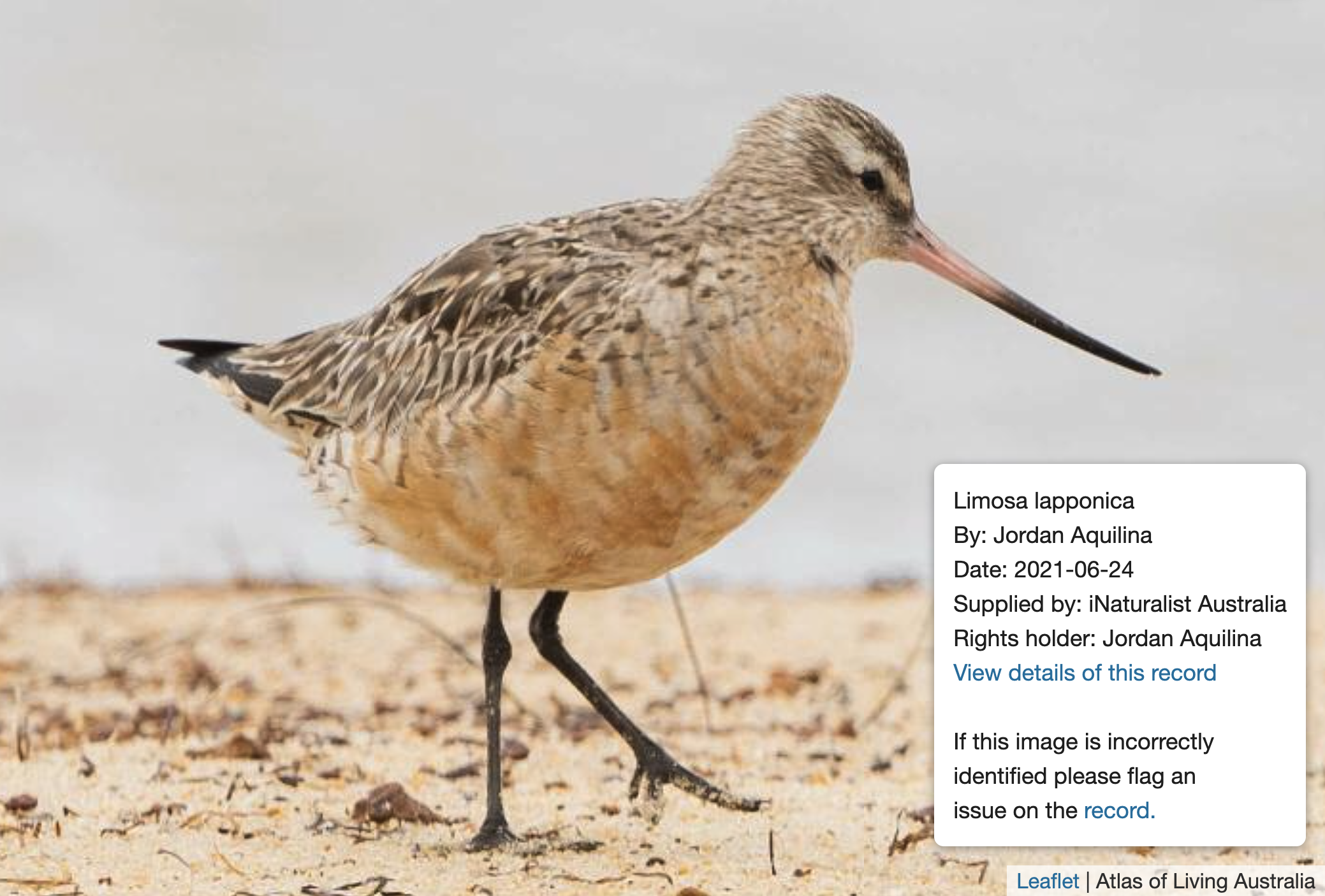
• Bar-tailed Godwit (Limosa lapponica) — Green #509E2F
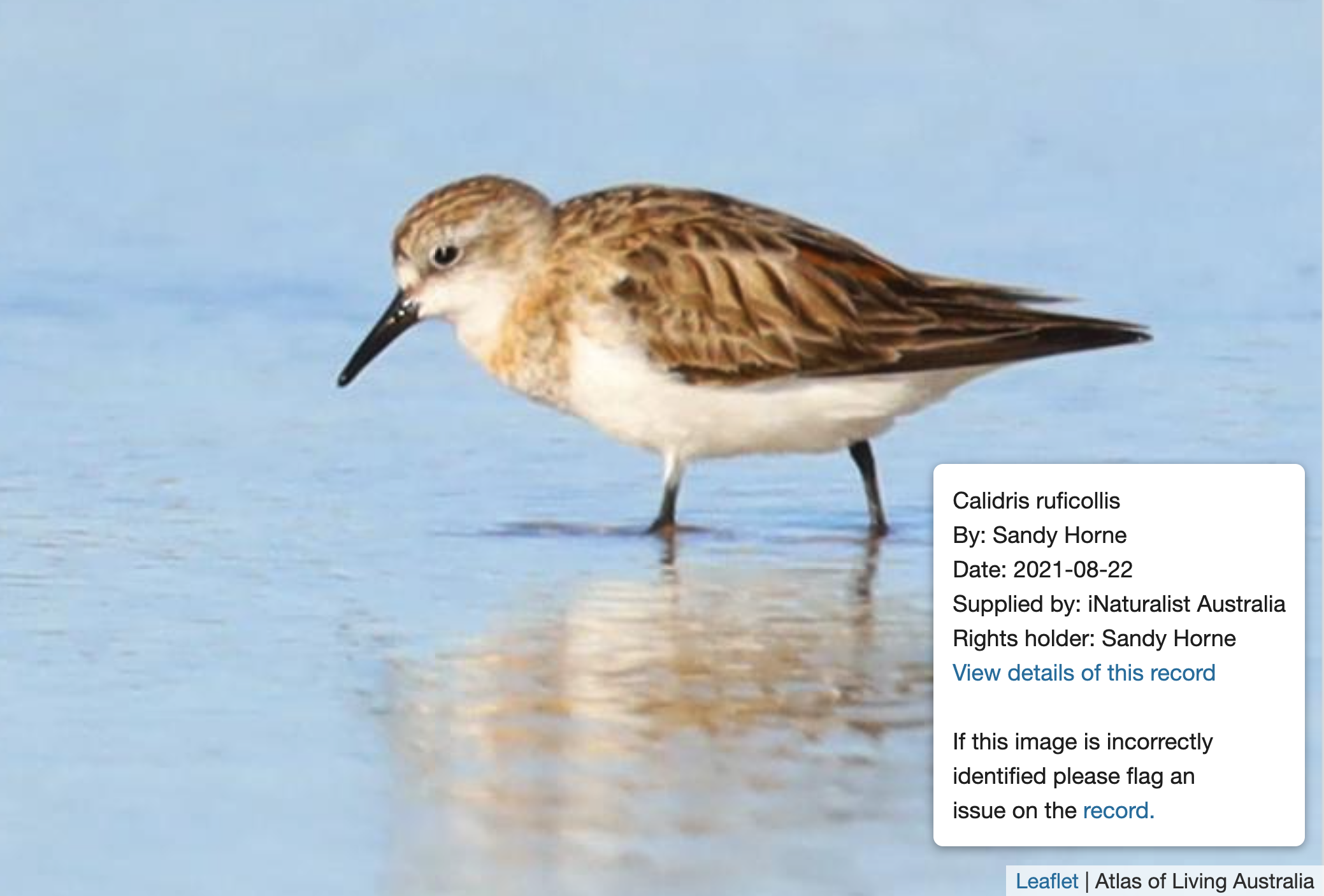
• Red-necked Stint (Calidris ruficollis) — Blue #2F6C99
• Curlew Sandpiper (Calidris ferruginea) — Orange #F39200

Each year, Australia welcomes millions of migratory species—from delicate shorebirds to majestic seabirds—journeying thousands of kilometres along flyways like the East Asian–Australasian Flyway.

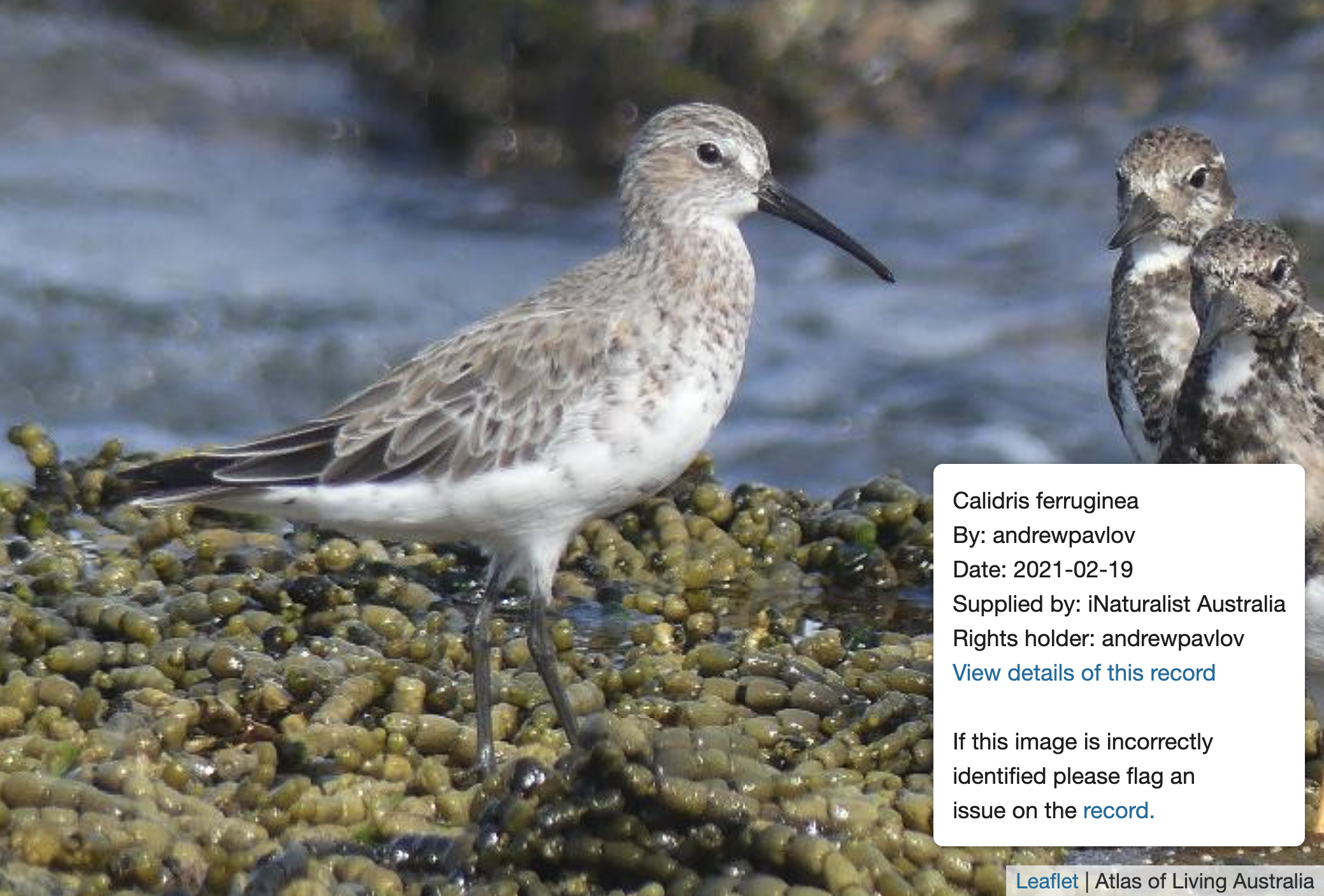
Species such as the Bar-tailed Godwit, Red-necked Stint, and Curlew Sandpiper arrive from as far as Siberia and Alaska, using Australia’s rich wetlands as critical stopovers and overwintering sites. These incredible travellers embody the resilience of nature and highlight the importance of conserving international migratory routes and coastal habitats.

Objectives:

Step	Description
1. Set the Working Directory	Prepare the environment and load necessary R packages.
2. Get Data	Retrieve occurrence data for target shorebird species from GBIF, iNaturalist, and OBIS. Merge all sources together.
3. Data Cleaning and Filtering	Clean the data, remove invalid points, and restrict to Australia’s boundary.
4. Data Visualisation	Visualize cleaned occurrences interactively using Leaflet maps with species-specific colours assigned explicitly to each species.
5. Save Data	Save the final datasets as CSV and Shapefile inside the data/ folder.

In the near future, this material may form part of comprehensive support materials available to EcoCommons users. If you have any corrections or suggestions to improve the efficiency, please contact the EcoCommons team.

Step 1: Set the working directory

Set the working directory and prepare the environment. Install necessary packages if missing and load them.

workspace <- getwd()
options(repr.plot.width = 16, repr.plot.height = 8)

options(repos = c(CRAN = "https://cran.rstudio.com/"))
packages <- c("spocc", "tidyverse", "pbapply", "leaflet", "sf", "rnaturalearth", "rnaturalearthdata")

for (pkg in packages) {
  if (!requireNamespace(pkg, quietly = TRUE)) {
    install.packages(pkg)
  }
  library(pkg, character.only = TRUE)
}

── Attaching core tidyverse packages ──────────────────────── tidyverse 2.0.0 ──
✔ dplyr     1.1.4     ✔ readr     2.1.5
✔ forcats   1.0.0     ✔ stringr   1.5.1
✔ ggplot2   3.5.2     ✔ tibble    3.2.1
✔ lubridate 1.9.4     ✔ tidyr     1.3.1
✔ purrr     1.0.4     
── Conflicts ────────────────────────────────────────── tidyverse_conflicts() ──
✖ dplyr::filter() masks stats::filter()
✖ dplyr::lag()    masks stats::lag()
ℹ Use the conflicted package (<http://conflicted.r-lib.org/>) to force all conflicts to become errors
Linking to GEOS 3.13.0, GDAL 3.8.5, PROJ 9.5.1; sf_use_s2() is TRUE


Attaching package: 'rnaturalearthdata'


The following object is masked from 'package:rnaturalearth':

    countries110

Step 2: Get Data

We define the target species and retrieve occurrence data from GBIF, iNaturalist, and OBIS. We combine all sources together into a single tidy data-frame for further processing.

species_list <- c("Limosa lapponica", "Calidris ruficollis", "Calidris ferruginea")

species_data <- pblapply(species_list, function(species) {
  occ(query = species, from = c("gbif", "inat", "obis"), limit = 500)
})

2 
3 
2 
3 
2 
3 

species_dfs <- lapply(species_data, function(data) {
  gbif_df <- occ2df(data$gbif)
  inat_df <- occ2df(data$inat)
  obis_df <- occ2df(data$obis)

  # Keep only longitude, latitude, name
  gbif_df <- gbif_df %>% select(longitude, latitude, name)
  inat_df <- inat_df %>% select(longitude, latitude, name)
  obis_df <- obis_df %>% select(longitude, latitude, name)

  # Make sure longitude and latitude are numeric
  gbif_df$longitude <- as.numeric(gbif_df$longitude)
  gbif_df$latitude  <- as.numeric(gbif_df$latitude)
  inat_df$longitude <- as.numeric(inat_df$longitude)
  inat_df$latitude  <- as.numeric(inat_df$latitude)
  obis_df$longitude <- as.numeric(obis_df$longitude)
  obis_df$latitude  <- as.numeric(obis_df$latitude)

  bind_rows(gbif_df, inat_df, obis_df)
})

for (i in seq_along(species_dfs)) {
  species_dfs[[i]]$species <- species_list[i]
}

occurrences <- bind_rows(species_dfs)

for (i in seq_along(species_list)) {
  cat("\nPreview of", species_list[i], "data:\n")
  print(head(species_dfs[[i]], 10))
}

Preview of Limosa lapponica data:
# A tibble: 10 × 4
   longitude latitude name                              species         
       <dbl>    <dbl> <chr>                             <chr>           
 1    153.      -27.3 Limosa lapponica (Linnaeus, 1758) Limosa lapponica
 2    153.      -27.3 Limosa lapponica (Linnaeus, 1758) Limosa lapponica
 3     -9.09     38.8 Limosa lapponica (Linnaeus, 1758) Limosa lapponica
 4    151.      -34.9 Limosa lapponica (Linnaeus, 1758) Limosa lapponica
 5      9.03     39.2 Limosa lapponica (Linnaeus, 1758) Limosa lapponica
 6    175.      -40.7 Limosa lapponica (Linnaeus, 1758) Limosa lapponica
 7    173.      -43.6 Limosa lapponica (Linnaeus, 1758) Limosa lapponica
 8    102.       12.7 Limosa lapponica (Linnaeus, 1758) Limosa lapponica
 9    102.       12.7 Limosa lapponica (Linnaeus, 1758) Limosa lapponica
10     72.9      18.8 Limosa lapponica (Linnaeus, 1758) Limosa lapponica

Preview of Calidris ruficollis data:
# A tibble: 10 × 4
   longitude latitude name                               species            
       <dbl>    <dbl> <chr>                              <chr>              
 1      145.    -38.0 Calidris ruficollis (Pallas, 1776) Calidris ruficollis
 2      145.    -38.0 Calidris ruficollis (Pallas, 1776) Calidris ruficollis
 3      153.    -27.7 Calidris ruficollis (Pallas, 1776) Calidris ruficollis
 4      151.    -33.7 Calidris ruficollis (Pallas, 1776) Calidris ruficollis
 5      151.    -34.9 Calidris ruficollis (Pallas, 1776) Calidris ruficollis
 6      151.    -34.9 Calidris ruficollis (Pallas, 1776) Calidris ruficollis
 7      145.    -38.0 Calidris ruficollis (Pallas, 1776) Calidris ruficollis
 8      145.    -38.5 Calidris ruficollis (Pallas, 1776) Calidris ruficollis
 9      145.    -38.5 Calidris ruficollis (Pallas, 1776) Calidris ruficollis
10      153.    -27.4 Calidris ruficollis (Pallas, 1776) Calidris ruficollis

Preview of Calidris ferruginea data:
# A tibble: 10 × 4
   longitude latitude name                                    species           
       <dbl>    <dbl> <chr>                                   <chr>             
 1    153.      -27.4 Calidris ferruginea (Pontoppidan, 1763) Calidris ferrugin…
 2    153.      -27.4 Calidris ferruginea (Pontoppidan, 1763) Calidris ferrugin…
 3    153.      -27.4 Calidris ferruginea (Pontoppidan, 1763) Calidris ferrugin…
 4     -7.74     37.1 Calidris ferruginea (Pontoppidan, 1763) Calidris ferrugin…
 5    145.      -38.0 Calidris ferruginea (Pontoppidan, 1763) Calidris ferrugin…
 6     70.2      22.5 Calidris ferruginea (Pontoppidan, 1763) Calidris ferrugin…
 7    153.      -27.4 Calidris ferruginea (Pontoppidan, 1763) Calidris ferrugin…
 8    116.      -32.6 Calidris ferruginea (Pontoppidan, 1763) Calidris ferrugin…
 9     25.6     -33.9 Calidris ferruginea (Pontoppidan, 1763) Calidris ferrugin…
10    145.      -38.0 Calidris ferruginea (Pontoppidan, 1763) Calidris ferrugin…

Step 3: Data Cleaning and Filtering

We clean the data by removing missing coordinates and converting points into spatial format. We then filter records to only those falling within Australia’s political boundaries.

occurrences_clean <- occurrences %>%
  filter(!is.na(longitude) & !is.na(latitude))

australia <- ne_countries(scale = "medium", returnclass = "sf") %>% filter(admin == "Australia")

occurrences_sf <- st_as_sf(occurrences_clean, coords = c("longitude", "latitude"), crs = 4326, remove = FALSE)

occurrences_aus <- st_intersection(occurrences_sf, australia)

Warning: attribute variables are assumed to be spatially constant throughout
all geometries

occurrences_aus <- occurrences_aus %>%
  select(longitude, latitude, species, geometry)

print(nrow(occurrences_aus))

[1] 1772

print(head(occurrences_aus))

Simple feature collection with 6 features and 3 fields
Geometry type: POINT
Dimension:     XY
Bounding box:  xmin: 150.7484 ymin: -34.8567 xmax: 153.1854 ymax: -27.30529
Geodetic CRS:  WGS 84
# A tibble: 6 × 4
  longitude latitude species                      geometry
      <dbl>    <dbl> <chr>                     <POINT [°]>
1      153.    -27.3 Limosa lapponica  (153.0949 -27.3413)
2      153.    -27.3 Limosa lapponica (153.0945 -27.34109)
3      151.    -34.9 Limosa lapponica  (150.7484 -34.8567)
4      153.    -27.3 Limosa lapponica (153.0704 -27.30529)
5      151.    -34.0 Limosa lapponica  (151.1259 -34.0158)
6      153.    -27.4 Limosa lapponica (153.1854 -27.44608)

Step 4: Data Visualisation

We use Leaflet to plot the cleaned occurrences on an interactive map. Each species is colour-coded by directly mapping species names to specific colours.

species_color_map <- c(
  "Limosa lapponica" = "#509E2F",
  "Calidris ruficollis" = "#2F6C99",
  "Calidris ferruginea" = "#F39200"
)

occurrences_aus$color <- unname(species_color_map[occurrences_aus$species])

leaflet(data = occurrences_aus) %>%
  addTiles() %>%
  addCircleMarkers(
    ~longitude, ~latitude,
    radius = 3, color = ~color,
    popup = ~species
  ) %>%
  addProviderTiles(providers$Esri.WorldImagery) %>%
  addLegend(
    "bottomright",
    colors = unname(species_color_map),
    labels = names(species_color_map),
    title = "Species"
  )

Step 5: Save Data

We save the final occurrence data-set as both CSV and Shape-file. The files are stored in a “data” folder to support further analysis or GIS integration.

if (!dir.exists("data")) {
  dir.create("data")
}

write.csv(occurrences_aus, "data/shorebird_occurrences_AUS.csv", row.names = FALSE)

if (!inherits(occurrences_aus, "sf")) {
  occurrences_aus <- st_as_sf(occurrences_aus, coords = c("longitude", "latitude"), crs = 4326, remove = FALSE)
}

st_write(occurrences_aus, "data/shorebird_occurrences_AUS.shp", delete_layer = TRUE)

Deleting layer `shorebird_occurrences_AUS' using driver `ESRI Shapefile'
Writing layer `shorebird_occurrences_AUS' to data source 
  `data/shorebird_occurrences_AUS.shp' using driver `ESRI Shapefile'
Writing 1772 features with 4 fields and geometry type Point.

References

• Owens, H., Barve, V., Chamberlain, S. (2025). spocc: Interface to Species Occurrence Data Sources. R package version 1.2.3. Available at: https://docs.ropensci.org/spocc/ and https://github.com/ropensci/spocc
• Chamberlain, S., Barve, V., Mcglinn, D., Oldoni, D., Desmet, P., Geffert, L., & Ram, K. (2024). spocc: Interface to Species Occurrence Data Sources. R package version 1.2.4. Available at: https://CRAN.R-project.org/package=spocc
• Wickham, H., Averick, M., Bryan, J., Chang, W., McGowan, L.D., François, R., et al. (2019). Welcome to the tidyverse. Journal of Open Source Software, 4(43), 1686. https://doi.org/10.21105/joss.01686
• Cheng, J., Karambelkar, B., Xie, Y. (2023). leaflet: Create Interactive Web Maps with the JavaScript ‘Leaflet’ Library. R package version 2.1.2.
• Pebesma, E. (2018). Simple Features for R: Standardized Support for Spatial Vector Data. The R Journal, 10(1), 439–446. https://doi.org/10.32614/RJ-2018-009
• South, A. (2017). rnaturalearth: World Map Data from Natural Earth. R package version 0.1.0.
• South, A. (2017). rnaturalearthdata: World Vector Map Data from Natural Earth Used in ‘rnaturalearth’. R package version 0.1.0.